Accessing Argo data by date using Argopy

also allows to download and represente the data by date. In this notebook we show a few examples, but we refer to the argopy Gallery for a more detailled explanation

Fist, as usual, import the libraries:

import numpy as np
import matplotlib as mpl
from matplotlib import pyplot as plt

import cartopy.crs as ccrs
import cartopy

import xarray as xr
xr.set_options(display_expand_attrs = False)

<xarray.core.options.set_options at 0x127a63a10>

Import argopy and set-up a data fetcher:

import argopy
from argopy.plot import scatter_map, scatter_plot  # Functions to easily make maps and plots

argopy.reset_options()
argopy.clear_cache()

You can load profiles for a specific date (and domain) using the region access point and specificating the region (-180, 180, -90, 90), the depth range (0, 100) and the date range (‘2020-11-11’, ‘2020-11-12’)

with argopy.set_options(parallel=True):
    params = 'all'  # eg: 'DOXY' or ['DOXY', 'BBP700']
    f = argopy.DataFetcher(params=params)
    f = f.region([-180, 180, -60, 60,0, 100,'2011-11-11','2011-11-22'])
    f.load()

f

<datafetcher.erddap>
⭐ Name: Ifremer erddap Argo data fetcher for a space/time region
🗺  Domain: [x=-180.00/180.00; y=-60.00/60.00; z=0.0/100.0; t=2011-11-11/2011-11-22]
🔗 API: https://erddap.ifremer.fr/erddap
🏊 User mode: standard
🟡+🔵 Dataset: phy
🌤  Performances: cache=False, parallel=True [thread]

apDS = f.data

apDS

<xarray.Dataset> Size: 8MB
Dimensions:          (N_POINTS: 69276)
Coordinates:
    LATITUDE         (N_POINTS) float64 554kB -51.79 -51.79 -51.79 ... 44.7 44.7
    LONGITUDE        (N_POINTS) float64 554kB -162.0 -162.0 ... 179.0 179.0
    TIME             (N_POINTS) datetime64[ns] 554kB 2011-11-11T02:59:21 ... ...
  * N_POINTS         (N_POINTS) int64 554kB 0 1 2 3 ... 69272 69273 69274 69275
Data variables: (12/15)
    CYCLE_NUMBER     (N_POINTS) int64 554kB 106 106 106 106 ... 126 126 126 126
    DATA_MODE        (N_POINTS) <U1 277kB 'D' 'D' 'D' 'D' ... 'D' 'D' 'D' 'D'
    DIRECTION        (N_POINTS) <U1 277kB 'A' 'A' 'A' 'A' ... 'A' 'A' 'A' 'A'
    PLATFORM_NUMBER  (N_POINTS) int64 554kB 5901691 5901691 ... 2900741 2900741
    POSITION_QC      (N_POINTS) int64 554kB 1 1 1 1 1 1 1 1 ... 1 1 1 1 1 1 1 1
    PRES             (N_POINTS) float32 277kB 5.7 9.9 20.4 ... 89.7 94.1 99.4
    ...               ...
    PSAL_ERROR       (N_POINTS) float32 277kB 0.01 0.01 0.01 ... 0.013 0.01 0.01
    PSAL_QC          (N_POINTS) int64 554kB 1 1 1 1 1 1 1 1 ... 1 1 1 1 1 1 1 1
    TEMP             (N_POINTS) float32 277kB 7.394 7.395 7.395 ... 11.14 10.57
    TEMP_ERROR       (N_POINTS) float32 277kB 0.002 0.002 0.002 ... 0.002 0.002
    TEMP_QC          (N_POINTS) int64 554kB 1 1 1 1 1 1 1 1 ... 1 1 1 1 1 1 1 1
    TIME_QC          (N_POINTS) int64 554kB 1 1 1 1 1 1 1 1 ... 1 1 1 1 1 1 1 1
Attributes: (8)

xarray.Dataset

• Dimensions:
  • N_POINTS: 69276
• Coordinates: (4)
  • LATITUDE
    (N_POINTS)
    float64
    -51.79 -51.79 -51.79 ... 44.7 44.7

    long_name :

    Latitude of the station, best estimate

    standard_name :

    latitude

    axis :

    Y

    valid_min :

    -90.0

    valid_max :

    90.0

    casted :

    1

    array([-51.792, -51.792, -51.792, ...,  44.7  ,  44.7  ,  44.7  ],
          shape=(69276,))

  • LONGITUDE
    (N_POINTS)
    float64
    -162.0 -162.0 ... 179.0 179.0

    long_name :

    Longitude of the station, best estimate

    standard_name :

    longitude

    axis :

    X

    valid_min :

    -180.0

    valid_max :

    180.0

    casted :

    1

    array([-161.991, -161.991, -161.991, ...,  178.992,  178.992,  178.992],
          shape=(69276,))

  • TIME
    (N_POINTS)
    datetime64[ns]
    2011-11-11T02:59:21 ... 2011-11-...

    _CoordinateAxisType :

    Time

    actual_range :

    [1.32098036e+09 1.32190795e+09]

    axis :

    T

    ioos_category :

    Time

    long_name :

    Julian day (UTC) of the station relative to REFERENCE_DATE_TIME

    standard_name :

    time

    time_origin :

    01-JAN-1970 00:00:00

    casted :

    1

    array(['2011-11-11T02:59:21.000000000', '2011-11-11T02:59:21.000000000',
           '2011-11-11T02:59:21.000000000', ...,
           '2011-11-21T23:17:32.000000000', '2011-11-21T23:17:32.000000000',
           '2011-11-21T23:17:32.000000000'],
          shape=(69276,), dtype='datetime64[ns]')

  • N_POINTS
    (N_POINTS)
    int64
    0 1 2 3 ... 69272 69273 69274 69275

    array([    0,     1,     2, ..., 69273, 69274, 69275], shape=(69276,))

• Data variables: (15)
  • CYCLE_NUMBER
    (N_POINTS)
    int64
    106 106 106 106 ... 126 126 126 126

    long_name :

    Float cycle number

    conventions :

    0..N, 0 : launch cycle (if exists), 1 : first complete cycle

    casted :

    1

    array([106, 106, 106, ..., 126, 126, 126], shape=(69276,))

  • DATA_MODE
    (N_POINTS)
    <U1
    'D' 'D' 'D' 'D' ... 'D' 'D' 'D' 'D'

    long_name :

    Delayed mode or real time data

    conventions :

    R : real time; D : delayed mode; A : real time with adjustment

    casted :

    1

    array(['D', 'D', 'D', ..., 'D', 'D', 'D'], shape=(69276,), dtype='<U1')

  • DIRECTION
    (N_POINTS)
    <U1
    'A' 'A' 'A' 'A' ... 'A' 'A' 'A' 'A'

    long_name :

    Direction of the station profiles

    conventions :

    A: ascending profiles, D: descending profiles

    casted :

    1

    array(['A', 'A', 'A', ..., 'A', 'A', 'A'], shape=(69276,), dtype='<U1')

  • PLATFORM_NUMBER
    (N_POINTS)
    int64
    5901691 5901691 ... 2900741 2900741

    long_name :

    Float unique identifier

    conventions :

    WMO float identifier : A9IIIII

    casted :

    1

    array([5901691, 5901691, 5901691, ..., 2900741, 2900741, 2900741],
          shape=(69276,))

  • POSITION_QC
    (N_POINTS)
    int64
    1 1 1 1 1 1 1 1 ... 1 1 1 1 1 1 1 1

    long_name :

    Global quality flag of POSITION_QC profile

    conventions :

    Argo reference table 2a

    casted :

    1

    array([1, 1, 1, ..., 1, 1, 1], shape=(69276,))

  • PRES
    (N_POINTS)
    float32
    5.7 9.9 20.4 ... 89.7 94.1 99.4

    long_name :

    Sea Pressure

    standard_name :

    sea_water_pressure

    units :

    decibar

    valid_min :

    0.0

    valid_max :

    12000.0

    resolution :

    0.1

    axis :

    Z

    casted :

    1

    array([ 5.7,  9.9, 20.4, ..., 89.7, 94.1, 99.4],
          shape=(69276,), dtype=float32)

  • PRES_ERROR
    (N_POINTS)
    float32
    2.4 2.4 2.4 2.4 ... 2.4 2.4 2.4 2.4

    long_name :

    ERROR IN Sea Pressure

    standard_name :

    sea_water_pressure

    units :

    decibar

    valid_min :

    0.0

    valid_max :

    12000.0

    resolution :

    0.1

    axis :

    Z

    casted :

    1

    array([2.4, 2.4, 2.4, ..., 2.4, 2.4, 2.4], shape=(69276,), dtype=float32)

  • PRES_QC
    (N_POINTS)
    int64
    1 1 1 1 1 1 1 1 ... 1 1 1 1 1 1 1 1

    long_name :

    Global quality flag of PRES_QC profile

    conventions :

    Argo reference table 2a

    casted :

    1

    array([1, 1, 1, ..., 1, 1, 1], shape=(69276,))

  • PSAL
    (N_POINTS)
    float32
    34.3 34.3 34.3 ... 33.81 33.99

    long_name :

    PRACTICAL SALINITY

    standard_name :

    sea_water_salinity

    units :

    psu

    valid_min :

    0.0

    valid_max :

    43.0

    resolution :

    0.001

    casted :

    1

    array([34.304, 34.304, 34.304, ..., 33.505, 33.814, 33.995],
          shape=(69276,), dtype=float32)

  • PSAL_ERROR
    (N_POINTS)
    float32
    0.01 0.01 0.01 ... 0.013 0.01 0.01

    long_name :

    ERROR IN PRACTICAL SALINITY

    standard_name :

    sea_water_salinity

    units :

    psu

    valid_min :

    0.0

    valid_max :

    43.0

    resolution :

    0.001

    casted :

    1

    array([0.01 , 0.01 , 0.01 , ..., 0.013, 0.01 , 0.01 ],
          shape=(69276,), dtype=float32)

  • PSAL_QC
    (N_POINTS)
    int64
    1 1 1 1 1 1 1 1 ... 1 1 1 1 1 1 1 1

    long_name :

    Global quality flag of PSAL_QC profile

    conventions :

    Argo reference table 2a

    casted :

    1

    array([1, 1, 1, ..., 1, 1, 1], shape=(69276,))

  • TEMP
    (N_POINTS)
    float32
    7.394 7.395 7.395 ... 11.14 10.57

    long_name :

    SEA TEMPERATURE IN SITU ITS-90 SCALE

    standard_name :

    sea_water_temperature

    units :

    degree_Celsius

    valid_min :

    -2.0

    valid_max :

    40.0

    resolution :

    0.001

    casted :

    1

    array([ 7.394,  7.395,  7.395, ..., 12.51 , 11.143, 10.566],
          shape=(69276,), dtype=float32)

  • TEMP_ERROR
    (N_POINTS)
    float32
    0.002 0.002 0.002 ... 0.002 0.002

    long_name :

    ERROR IN SEA TEMPERATURE IN SITU ITS-90 SCALE

    standard_name :

    sea_water_temperature

    units :

    degree_Celsius

    valid_min :

    -2.0

    valid_max :

    40.0

    resolution :

    0.001

    casted :

    1

    array([0.002, 0.002, 0.002, ..., 0.002, 0.002, 0.002],
          shape=(69276,), dtype=float32)

  • TEMP_QC
    (N_POINTS)
    int64
    1 1 1 1 1 1 1 1 ... 1 1 1 1 1 1 1 1

    long_name :

    Global quality flag of TEMP_QC profile

    conventions :

    Argo reference table 2a

    casted :

    1

    array([1, 1, 1, ..., 1, 1, 1], shape=(69276,))

  • TIME_QC
    (N_POINTS)
    int64
    1 1 1 1 1 1 1 1 ... 1 1 1 1 1 1 1 1

    long_name :

    Global quality flag of TIME_QC profile

    conventions :

    Argo reference table 2a

    casted :

    1

    array([1, 1, 1, ..., 1, 1, 1], shape=(69276,))

• Indexes: (1)
  • N_POINTS
    PandasIndex

    PandasIndex(Index([    0,     1,     2,     3,     4,     5,     6,     7,     8,     9,
           ...
           69266, 69267, 69268, 69269, 69270, 69271, 69272, 69273, 69274, 69275],
          dtype='int64', name='N_POINTS', length=69276))

• Attributes: (8)

  DATA_ID :

  ARGO

  DOI :

  http://doi.org/10.17882/42182

  Fetched_from :

  erddap.ifremer.fr

  Fetched_by :

  pvb

  Fetched_date :

  2025/09/19

  Fetched_constraints :

  [x=-180.00/-160.00; y=-60.00/-40.00; z=0.0/100.0; t=2011-11-11/2011-11-22]

  Fetched_uri :

  https://erddap.ifremer.fr/erddap/tabledap/ArgoFloats.nc?config_mission_number,cycle_number,data_mode,direction,latitude,longitude,platform_number,position_qc,pres,pres_adjusted,pres_adjusted_error,pres_adjusted_qc,pres_qc,psal,psal_adjusted,psal_adjusted_error,psal_adjusted_qc,psal_qc,temp,temp_adjusted,temp_adjusted_error,temp_adjusted_qc,temp_qc,time,time_qc,vertical_sampling_scheme&longitude%3E=-180.0&longitude%3C=-160.0&latitude%3E=-60.0&latitude%3C=-40.0&pres%3E=0&pres%3C=100&time%3E=1320969600.0&time%3C=1321920000.0&latitude!=NaN&longitude!=NaN&distinct()&orderBy(%22time,pres%22)

  Processing_history :

  [PRES,TEMP,PSAL] real-time and adjusted/delayed variables merged according to their data mode; [POSITION_QC,PRES_QC,PSAL_QC,TEMP_QC,TIME_QC] filtered to retain points with QC in [1,2]

note that the data is organized in ‘points’, a 1D array collection of measurements:

apDS.TEMP

<xarray.DataArray 'TEMP' (N_POINTS: 69276)> Size: 277kB
array([ 7.394,  7.395,  7.395, ..., 12.51 , 11.143, 10.566],
      shape=(69276,), dtype=float32)
Coordinates:
    LATITUDE   (N_POINTS) float64 554kB -51.79 -51.79 -51.79 ... 44.7 44.7 44.7
    LONGITUDE  (N_POINTS) float64 554kB -162.0 -162.0 -162.0 ... 179.0 179.0
    TIME       (N_POINTS) datetime64[ns] 554kB 2011-11-11T02:59:21 ... 2011-1...
  * N_POINTS   (N_POINTS) int64 554kB 0 1 2 3 4 ... 69272 69273 69274 69275
Attributes: (7)

xarray.DataArray

'TEMP'

• N_POINTS: 69276

• 7.394 7.395 7.395 7.396 7.381 7.352 ... 12.56 12.56 12.51 11.14 10.57

  array([ 7.394,  7.395,  7.395, ..., 12.51 , 11.143, 10.566],
        shape=(69276,), dtype=float32)

• Coordinates: (4)
  • LATITUDE
    (N_POINTS)
    float64
    -51.79 -51.79 -51.79 ... 44.7 44.7

    long_name :

    Latitude of the station, best estimate

    standard_name :

    latitude

    axis :

    Y

    valid_min :

    -90.0

    valid_max :

    90.0

    casted :

    1

    array([-51.792, -51.792, -51.792, ...,  44.7  ,  44.7  ,  44.7  ],
          shape=(69276,))

  • LONGITUDE
    (N_POINTS)
    float64
    -162.0 -162.0 ... 179.0 179.0

    long_name :

    Longitude of the station, best estimate

    standard_name :

    longitude

    axis :

    X

    valid_min :

    -180.0

    valid_max :

    180.0

    casted :

    1

    array([-161.991, -161.991, -161.991, ...,  178.992,  178.992,  178.992],
          shape=(69276,))

  • TIME
    (N_POINTS)
    datetime64[ns]
    2011-11-11T02:59:21 ... 2011-11-...

    _CoordinateAxisType :

    Time

    actual_range :

    [1.32098036e+09 1.32190795e+09]

    axis :

    T

    ioos_category :

    Time

    long_name :

    Julian day (UTC) of the station relative to REFERENCE_DATE_TIME

    standard_name :

    time

    time_origin :

    01-JAN-1970 00:00:00

    casted :

    1

    array(['2011-11-11T02:59:21.000000000', '2011-11-11T02:59:21.000000000',
           '2011-11-11T02:59:21.000000000', ...,
           '2011-11-21T23:17:32.000000000', '2011-11-21T23:17:32.000000000',
           '2011-11-21T23:17:32.000000000'],
          shape=(69276,), dtype='datetime64[ns]')

  • N_POINTS
    (N_POINTS)
    int64
    0 1 2 3 ... 69272 69273 69274 69275

    array([    0,     1,     2, ..., 69273, 69274, 69275], shape=(69276,))

• Indexes: (1)
  • N_POINTS
    PandasIndex

    PandasIndex(Index([    0,     1,     2,     3,     4,     5,     6,     7,     8,     9,
           ...
           69266, 69267, 69268, 69269, 69270, 69271, 69272, 69273, 69274, 69275],
          dtype='int64', name='N_POINTS', length=69276))

• Attributes: (7)

  long_name :

  SEA TEMPERATURE IN SITU ITS-90 SCALE

  standard_name :

  sea_water_temperature

  units :

  degree_Celsius

  valid_min :

  -2.0

  valid_max :

  40.0

  resolution :

  0.001

  casted :

  1

However, and for the purpose of the Argo online school is easier to work with the data in profiles; argopy allows the transformation:

data=apDS.argo.point2profile()
data

<xarray.Dataset> Size: 8MB
Dimensions:          (N_PROF: 3396, N_LEVELS: 99)
Coordinates:
  * N_PROF           (N_PROF) int64 27kB 2838 124 874 2061 ... 3350 1957 3176
  * N_LEVELS         (N_LEVELS) int64 792B 0 1 2 3 4 5 6 ... 93 94 95 96 97 98
    LATITUDE         (N_PROF) float64 27kB 29.51 -54.95 9.267 ... -52.37 43.28
    LONGITUDE        (N_PROF) float64 27kB -144.0 70.81 87.32 ... -138.6 7.668
    TIME             (N_PROF) datetime64[ns] 27kB 2011-11-11T00:06:10 ... 201...
Data variables: (12/15)
    CYCLE_NUMBER     (N_PROF) int64 27kB 2 183 76 186 134 ... 137 233 19 198 192
    DATA_MODE        (N_PROF) <U1 14kB 'D' 'D' 'D' 'D' 'D' ... 'D' 'D' 'D' 'D'
    DIRECTION        (N_PROF) <U1 14kB 'A' 'A' 'A' 'A' 'A' ... 'A' 'A' 'A' 'A'
    PLATFORM_NUMBER  (N_PROF) int64 27kB 5903597 1900927 ... 5901067 6900699
    POSITION_QC      (N_PROF) int64 27kB 1 1 1 1 1 1 1 1 1 ... 1 1 1 1 1 1 1 1 1
    PRES             (N_PROF, N_LEVELS) float32 1MB 6.2 9.5 19.4 ... nan nan nan
    ...               ...
    PSAL_ERROR       (N_PROF, N_LEVELS) float32 1MB 0.01 0.01 0.01 ... nan nan
    PSAL_QC          (N_PROF) int64 27kB 1 1 1 1 1 1 1 1 2 ... 1 1 1 1 1 1 1 1 1
    TEMP             (N_PROF, N_LEVELS) float32 1MB 22.57 22.56 ... nan nan
    TEMP_ERROR       (N_PROF, N_LEVELS) float32 1MB 0.002 0.002 ... nan nan
    TEMP_QC          (N_PROF) int64 27kB 1 1 1 1 1 1 1 1 2 ... 1 1 1 1 1 1 1 1 1
    TIME_QC          (N_PROF) int64 27kB 1 1 1 1 1 1 1 1 1 ... 2 1 1 1 1 1 1 1 1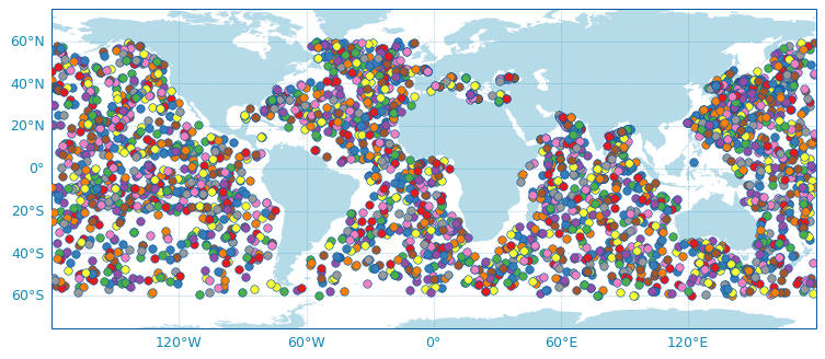
Attributes: (8)

xarray.Dataset

• Dimensions:
  • N_PROF: 3396
  • N_LEVELS: 99
• Coordinates: (5)
  • N_PROF
    (N_PROF)
    int64
    2838 124 874 ... 3350 1957 3176

    casted :

    1

    array([2838,  124,  874, ..., 3350, 1957, 3176], shape=(3396,))

  • N_LEVELS
    (N_LEVELS)
    int64
    0 1 2 3 4 5 6 ... 93 94 95 96 97 98

    casted :

    1

    array([ 0,  1,  2,  3,  4,  5,  6,  7,  8,  9, 10, 11, 12, 13, 14, 15, 16, 17,
           18, 19, 20, 21, 22, 23, 24, 25, 26, 27, 28, 29, 30, 31, 32, 33, 34, 35,
           36, 37, 38, 39, 40, 41, 42, 43, 44, 45, 46, 47, 48, 49, 50, 51, 52, 53,
           54, 55, 56, 57, 58, 59, 60, 61, 62, 63, 64, 65, 66, 67, 68, 69, 70, 71,
           72, 73, 74, 75, 76, 77, 78, 79, 80, 81, 82, 83, 84, 85, 86, 87, 88, 89,
           90, 91, 92, 93, 94, 95, 96, 97, 98])

  • LATITUDE
    (N_PROF)
    float64
    29.51 -54.95 9.267 ... -52.37 43.28

    long_name :

    Latitude of the station, best estimate

    standard_name :

    latitude

    axis :

    Y

    valid_min :

    -90.0

    valid_max :

    90.0

    casted :

    1

    array([ 29.509, -54.949,   9.267, ...,  22.348, -52.37 ,  43.276],
          shape=(3396,))

  • LONGITUDE
    (N_PROF)
    float64
    -144.0 70.81 87.32 ... -138.6 7.668

    long_name :

    Longitude of the station, best estimate

    standard_name :

    longitude

    axis :

    X

    valid_min :

    -180.0

    valid_max :

    180.0

    casted :

    1

    array([-143.987,   70.807,   87.322, ...,  -53.078, -138.647,    7.668],
          shape=(3396,))

  • TIME
    (N_PROF)
    datetime64[ns]
    2011-11-11T00:06:10 ... 2011-11-22

    _CoordinateAxisType :

    Time

    actual_range :

    [1.32098036e+09 1.32190795e+09]

    axis :

    T

    ioos_category :

    Time

    long_name :

    Julian day (UTC) of the station relative to REFERENCE_DATE_TIME

    standard_name :

    time

    time_origin :

    01-JAN-1970 00:00:00

    casted :

    1

    array(['2011-11-11T00:06:10.000000000', '2011-11-11T00:11:00.000000000',
           '2011-11-11T00:14:26.000000000', ...,
           '2011-11-21T23:49:21.000000000', '2011-11-21T23:59:53.000000000',
           '2011-11-22T00:00:00.000000000'],
          shape=(3396,), dtype='datetime64[ns]')

• Data variables: (15)
  • CYCLE_NUMBER
    (N_PROF)
    int64
    2 183 76 186 134 ... 233 19 198 192

    long_name :

    Float cycle number

    conventions :

    0..N, 0 : launch cycle (if exists), 1 : first complete cycle

    casted :

    1

    array([  2, 183,  76, ...,  19, 198, 192], shape=(3396,))

  • DATA_MODE
    (N_PROF)
    <U1
    'D' 'D' 'D' 'D' ... 'D' 'D' 'D' 'D'

    long_name :

    Delayed mode or real time data

    conventions :

    R : real time; D : delayed mode; A : real time with adjustment

    casted :

    1

    array(['D', 'D', 'D', ..., 'D', 'D', 'D'], shape=(3396,), dtype='<U1')

  • DIRECTION
    (N_PROF)
    <U1
    'A' 'A' 'A' 'A' ... 'A' 'A' 'A' 'A'

    long_name :

    Direction of the station profiles

    conventions :

    A: ascending profiles, D: descending profiles

    casted :

    1

    array(['A', 'A', 'A', ..., 'A', 'A', 'A'], shape=(3396,), dtype='<U1')

  • PLATFORM_NUMBER
    (N_PROF)
    int64
    5903597 1900927 ... 5901067 6900699

    long_name :

    Float unique identifier

    conventions :

    WMO float identifier : A9IIIII

    casted :

    1

    array([5903597, 1900927, 2901285, ..., 6901052, 5901067, 6900699],
          shape=(3396,))

  • POSITION_QC
    (N_PROF)
    int64
    1 1 1 1 1 1 1 1 ... 1 1 1 1 1 1 1 1

    long_name :

    Global quality flag of POSITION_QC profile

    conventions :

    Argo reference table 2a

    casted :

    1

    array([1, 1, 1, ..., 1, 1, 1], shape=(3396,))

  • PRES
    (N_PROF, N_LEVELS)
    float32
    6.2 9.5 19.4 29.5 ... nan nan nan

    long_name :

    Sea Pressure

    standard_name :

    sea_water_pressure

    units :

    decibar

    valid_min :

    0.0

    valid_max :

    12000.0

    resolution :

    0.1

    axis :

    Z

    casted :

    1

    array([[ 6.2,  9.5, 19.4, ...,  nan,  nan,  nan],
           [16. , 27. , 36. , ...,  nan,  nan,  nan],
           [ 4.8, 10.2, 15.2, ...,  nan,  nan,  nan],
           ...,
           [ 6.6, 10.7, 15.6, ...,  nan,  nan,  nan],
           [ 4.3,  9.1, 19. , ...,  nan,  nan,  nan],
           [ 8. , 13. , 18. , ...,  nan,  nan,  nan]],
          shape=(3396, 99), dtype=float32)

  • PRES_ERROR
    (N_PROF, N_LEVELS)
    float32
    2.4 2.4 2.4 2.4 ... nan nan nan nan

    long_name :

    ERROR IN Sea Pressure

    standard_name :

    sea_water_pressure

    units :

    decibar

    valid_min :

    0.0

    valid_max :

    12000.0

    resolution :

    0.1

    axis :

    Z

    casted :

    1

    array([[2.4, 2.4, 2.4, ..., nan, nan, nan],
           [2.4, 2.4, 2.4, ..., nan, nan, nan],
           [2.4, 2.4, 2.4, ..., nan, nan, nan],
           ...,
           [2.4, 2.4, 2.4, ..., nan, nan, nan],
           [2.4, 2.4, 2.4, ..., nan, nan, nan],
           [2.4, 2.4, 2.4, ..., nan, nan, nan]],
          shape=(3396, 99), dtype=float32)

  • PRES_QC
    (N_PROF)
    int64
    1 1 1 1 1 1 1 1 ... 1 1 1 1 1 1 1 1

    long_name :

    Global quality flag of PRES_QC profile

    conventions :

    Argo reference table 2a

    casted :

    1

    array([1, 1, 1, ..., 1, 1, 1], shape=(3396,))

  • PSAL
    (N_PROF, N_LEVELS)
    float32
    35.43 35.43 35.42 ... nan nan nan

    long_name :

    PRACTICAL SALINITY

    standard_name :

    sea_water_salinity

    units :

    psu

    valid_min :

    0.0

    valid_max :

    43.0

    resolution :

    0.001

    casted :

    1

    array([[35.42708, 35.42607, 35.42408, ...,      nan,      nan,      nan],
           [33.832  , 33.832  , 33.832  , ...,      nan,      nan,      nan],
           [33.151  , 33.151  , 33.159  , ...,      nan,      nan,      nan],
           ...,
           [36.13494, 36.13294, 36.12494, ...,      nan,      nan,      nan],
           [34.319  , 34.319  , 34.32   , ...,      nan,      nan,      nan],
           [38.135  , 38.135  , 38.133  , ...,      nan,      nan,      nan]],
          shape=(3396, 99), dtype=float32)

  • PSAL_ERROR
    (N_PROF, N_LEVELS)
    float32
    0.01 0.01 0.01 0.01 ... nan nan nan

    long_name :

    ERROR IN PRACTICAL SALINITY

    standard_name :

    sea_water_salinity

    units :

    psu

    valid_min :

    0.0

    valid_max :

    43.0

    resolution :

    0.001

    casted :

    1

    array([[0.01 , 0.01 , 0.01 , ...,   nan,   nan,   nan],
           [0.02 , 0.02 , 0.02 , ...,   nan,   nan,   nan],
           [0.01 , 0.01 , 0.01 , ...,   nan,   nan,   nan],
           ...,
           [0.01 , 0.01 , 0.01 , ...,   nan,   nan,   nan],
           [0.01 , 0.01 , 0.01 , ...,   nan,   nan,   nan],
           [0.005, 0.005, 0.005, ...,   nan,   nan,   nan]],
          shape=(3396, 99), dtype=float32)

  • PSAL_QC
    (N_PROF)
    int64
    1 1 1 1 1 1 1 1 ... 1 1 1 1 1 1 1 1

    long_name :

    Global quality flag of PSAL_QC profile

    conventions :

    Argo reference table 2a

    casted :

    1

    array([1, 1, 1, ..., 1, 1, 1], shape=(3396,))

  • TEMP
    (N_PROF, N_LEVELS)
    float32
    22.57 22.56 22.57 ... nan nan nan

    long_name :

    SEA TEMPERATURE IN SITU ITS-90 SCALE

    standard_name :

    sea_water_temperature

    units :

    degree_Celsius

    valid_min :

    -2.0

    valid_max :

    40.0

    resolution :

    0.001

    casted :

    1

    array([[22.565, 22.563, 22.565, ...,    nan,    nan,    nan],
           [ 1.321,  1.323,  1.323, ...,    nan,    nan,    nan],
           [29.029, 29.037, 29.044, ...,    nan,    nan,    nan],
           ...,
           [27.332, 27.32 , 27.282, ...,    nan,    nan,    nan],
           [ 7.595,  7.598,  7.609, ...,    nan,    nan,    nan],
           [16.288, 16.29 , 16.286, ...,    nan,    nan,    nan]],
          shape=(3396, 99), dtype=float32)

  • TEMP_ERROR
    (N_PROF, N_LEVELS)
    float32
    0.002 0.002 0.002 ... nan nan nan

    long_name :

    ERROR IN SEA TEMPERATURE IN SITU ITS-90 SCALE

    standard_name :

    sea_water_temperature

    units :

    degree_Celsius

    valid_min :

    -2.0

    valid_max :

    40.0

    resolution :

    0.001

    casted :

    1

    array([[0.002, 0.002, 0.002, ...,   nan,   nan,   nan],
           [0.002, 0.002, 0.002, ...,   nan,   nan,   nan],
           [0.002, 0.002, 0.002, ...,   nan,   nan,   nan],
           ...,
           [0.002, 0.002, 0.002, ...,   nan,   nan,   nan],
           [0.002, 0.002, 0.002, ...,   nan,   nan,   nan],
           [0.002, 0.002, 0.002, ...,   nan,   nan,   nan]],
          shape=(3396, 99), dtype=float32)

  • TEMP_QC
    (N_PROF)
    int64
    1 1 1 1 1 1 1 1 ... 1 1 1 1 1 1 1 1

    long_name :

    Global quality flag of TEMP_QC profile

    conventions :

    Argo reference table 2a

    casted :

    1

    array([1, 1, 1, ..., 1, 1, 1], shape=(3396,))

  • TIME_QC
    (N_PROF)
    int64
    1 1 1 1 1 1 1 1 ... 1 1 1 1 1 1 1 1

    long_name :

    Global quality flag of TIME_QC profile

    conventions :

    Argo reference table 2a

    casted :

    1

    array([1, 1, 1, ..., 1, 1, 1], shape=(3396,))

• Indexes: (2)
  • N_PROF
    PandasIndex

    PandasIndex(Index([2838,  124,  874, 2061,  105, 1895, 2479, 1599, 1806, 1677,
           ...
           2731, 1071, 3255,  795,  790, 2177, 1873, 3350, 1957, 3176],
          dtype='int64', name='N_PROF', length=3396))

  • N_LEVELS
    PandasIndex

    PandasIndex(Index([ 0,  1,  2,  3,  4,  5,  6,  7,  8,  9, 10, 11, 12, 13, 14, 15, 16, 17,
           18, 19, 20, 21, 22, 23, 24, 25, 26, 27, 28, 29, 30, 31, 32, 33, 34, 35,
           36, 37, 38, 39, 40, 41, 42, 43, 44, 45, 46, 47, 48, 49, 50, 51, 52, 53,
           54, 55, 56, 57, 58, 59, 60, 61, 62, 63, 64, 65, 66, 67, 68, 69, 70, 71,
           72, 73, 74, 75, 76, 77, 78, 79, 80, 81, 82, 83, 84, 85, 86, 87, 88, 89,
           90, 91, 92, 93, 94, 95, 96, 97, 98],
          dtype='int64', name='N_LEVELS'))

• Attributes: (8)

  DATA_ID :

  ARGO

  DOI :

  http://doi.org/10.17882/42182

  Fetched_from :

  erddap.ifremer.fr

  Fetched_by :

  pvb

  Fetched_date :

  2025/09/19

  Fetched_constraints :

  [x=-180.00/-160.00; y=-60.00/-40.00; z=0.0/100.0; t=2011-11-11/2011-11-22]

  Fetched_uri :

  https://erddap.ifremer.fr/erddap/tabledap/ArgoFloats.nc?config_mission_number,cycle_number,data_mode,direction,latitude,longitude,platform_number,position_qc,pres,pres_adjusted,pres_adjusted_error,pres_adjusted_qc,pres_qc,psal,psal_adjusted,psal_adjusted_error,psal_adjusted_qc,psal_qc,temp,temp_adjusted,temp_adjusted_error,temp_adjusted_qc,temp_qc,time,time_qc,vertical_sampling_scheme&longitude%3E=-180.0&longitude%3C=-160.0&latitude%3E=-60.0&latitude%3C=-40.0&pres%3E=0&pres%3C=100&time%3E=1320969600.0&time%3C=1321920000.0&latitude!=NaN&longitude!=NaN&distinct()&orderBy(%22time,pres%22)

  Processing_history :

  [PRES,TEMP,PSAL] real-time and adjusted/delayed variables merged according to their data mode; [POSITION_QC,PRES_QC,PSAL_QC,TEMP_QC,TIME_QC] filtered to retain points with QC in [1,2]; Transformed with 'point2profile'

and we can plot all the profiles measured during this month:

scatter_map(data,legend = False);

/Users/pvb/miniconda3/envs/AOS/lib/python3.13/site-packages/argopy/plot/plot.py:489: UserWarning: More than one N_LEVELS found in this dataset, scatter_map will use the first level only
  warnings.warn(

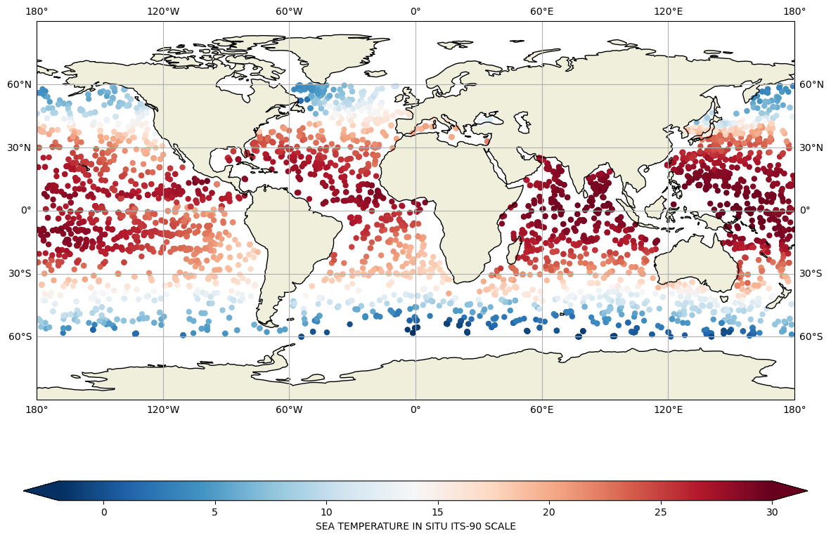
We can look at the upper 10db temperature values:

temp = apDS.where(apDS['PRES']<10)['TEMP']

lon=temp.LONGITUDE
lat=temp.LATITUDE

fig,ax = plt.subplots(figsize=(18,10),subplot_kw={'projection': ccrs.PlateCarree()})
ax.set_global()

# data for each basin
cs=ax.scatter(lon,lat,c=temp,cmap="RdBu_r",vmin=-2, vmax=30, edgecolor='none')

ax.coastlines()
ax.add_feature(cartopy.feature.LAND.with_scale('110m'))
ax.gridlines(draw_labels=True, x_inline=False, y_inline=False);

#colorbar
cbar=fig.colorbar(cs,ax=ax,extend='both',orientation='horizontal',shrink=.8,aspect=40)
cbar.set_label(temp.long_name)