Accessing all profiles at once

Accessing all profiles at once#

Conveniently, all the core mission profiles are compacted in a single file, named: <FloatWmoID>_prof.nc. However, some information is only in the individual profile files, but we will see it.

Let’s start loading the neccesary python modules and the netCDF file 6901254/6901254_prof.nc

import numpy as np
import xarray as xr
import netCDF4
from matplotlib import pyplot as plt
%matplotlib inline

prof  = xr.open_dataset('../../Data/202107-ArgoData/dac/coriolis/6901254/6901254_prof.nc')

In this case, N_PROF is 66, since there are 66 profiles, including two for the first cycle, the descending and the ascending. These profiles are just the ‘Primary sampling’, if you need the high-resolution upper 5 dbar you have to use the individual cycle files, LOADING ‘../../Data/202107-ArgoData/dac/coriolis/6901254/profiles/R6901254_001.nc’ as we saw in the previous chapter.

Let’s visualize all the salinity observations, a first a quick-look

fig , ax = plt.subplots(figsize=(10,10))
ax.contourf(prof.PSAL);

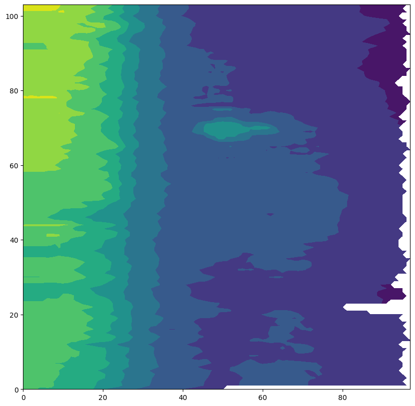
../../_images/383814d5696c34e7c7551733453524b680bef8b063ee8f3c30a876874ce9d5c7.png

However, we want to add the proper pressure levels since each profile has slightly different levels. For instance note the different values of the pressure observations for profile 3 and 4:

prof.PRES[3,:].values

array([   6.,    7.,    8.,    9.,   10.,   16.,   25.,   36.,   46.,
         55.,   66.,   76.,   86.,   96.,  106.,  115.,  125.,  135.,
        146.,  156.,  165.,  176.,  186.,  196.,  213.,  237.,  262.,
        288.,  313.,  338.,  363.,  388.,  413.,  438.,  463.,  488.,
        513.,  538.,  563.,  588.,  613.,  638.,  663.,  687.,  713.,
        738.,  763.,  788.,  813.,  838.,  863.,  888.,  914.,  938.,
        963.,  988., 1013., 1038., 1063., 1088., 1113., 1139., 1163.,
       1188., 1213., 1238., 1263., 1288., 1313., 1338., 1363., 1388.,
       1413., 1439., 1463., 1488., 1513., 1538., 1563., 1588., 1613.,
       1638., 1663., 1688., 1713., 1738., 1763., 1788., 1813., 1838.,
       1863., 1888., 1913., 1938., 1963., 1988., 2013., 2036.],
      dtype=float32)

prof.PRES[4,:].values

array([   6.,    7.,    8.,    9.,   10.,   16.,   25.,   35.,   45.,
         55.,   66.,   75.,   85.,   95.,  106.,  116.,  125.,  135.,
        145.,  156.,  165.,  175.,  186.,  196.,  213.,  238.,  263.,
        287.,  313.,  338.,  363.,  388.,  413.,  438.,  463.,  488.,
        513.,  538.,  563.,  588.,  613.,  638.,  663.,  689.,  713.,
        738.,  763.,  788.,  813.,  838.,  863.,  889.,  913.,  938.,
        963.,  988., 1013., 1038., 1063., 1089., 1113., 1138., 1163.,
       1188., 1213., 1238., 1263., 1289., 1313., 1338., 1363., 1388.,
       1413., 1438., 1462., 1488., 1513., 1538., 1563., 1588., 1613.,
       1639., 1663., 1688., 1713., 1737., 1763., 1788., 1813., 1837.,
       1863., 1888., 1913., 1938., 1963., 1978.,   nan,   nan],
      dtype=float32)

Therefore we need to do a little of interpolation into a common set of pressure values:

prei=np.arange(5,2005,5) # we define a common set of pressure values:

We define the new vectors

juld=prof.JULD.values
psal=prof.PSAL.values
temp=prof.TEMP.values
pres=prof.PRES.values

psali= np.zeros((juld.shape[0],prei.shape[0]))
psali.fill(np.nan)

tempi= np.zeros((juld.shape[0],prei.shape[0]))
tempi.fill(np.nan)

and then we interpolate the salinity and the temperature onto the new levels:

for ip in range(0,pres.shape[0]-1):
    psali[ip,:]=np.interp(prei,pres[ip,:],psal[ip,:])
    tempi[ip,:]=np.interp(prei,pres[ip,:],temp[ip,:])

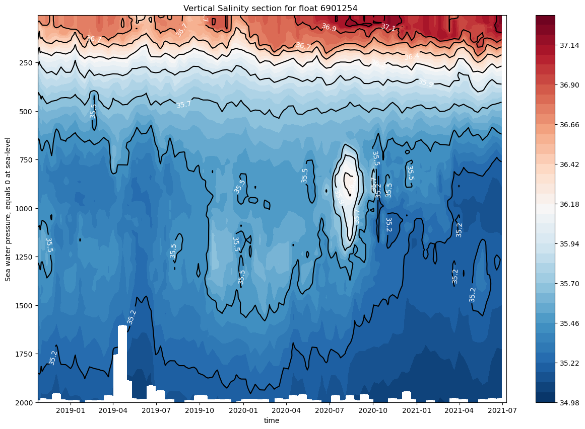
and let’s plot the time evolution of the saliniy measured by this float. in oceanography we usually call it a section

This figure is a little more complex, Unfortunatly we can not teach everything AoS, and therefore we do not explain all the python code, but if you want to get extra information, please make and issue in GitHub

fig, ax = plt.subplots(figsize=(15,10))

#Draw the contours for the salinity
cs=ax.contourf(juld,prei,psali.transpose(),40,cmap="RdBu_r")

#Draw the contours lines to be labelled
cs2=ax.contour(juld,prei,psali.transpose(),colors=('k'), levels=cs.levels[::4])

#Since pressure increase away from the surface we invert the y-axis
ax.invert_yaxis()
ax.clabel(cs2, fmt='%2.1f', colors='w', fontsize=10)

#Add the titles
ax.set_title(f"Vertical Salinity section for float {prof.PLATFORM_NUMBER[0].astype(str).values}")
ax.set_xlabel(f"{prof.JULD.standard_name}")
ax.set_ylabel(f"{prof.PRES.long_name}")

#Add the colorbar
cbar=fig.colorbar(cs,ax=ax)

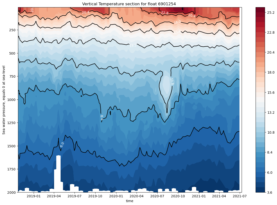
../../_images/26e3c7fc39109c0fa40f5ebefc9696f1701c28319d25ff913a88bf2950dc9fdb.png

And the same for temperature:

fig, ax = plt.subplots(figsize=(15,10))

cs=ax.contourf(juld,prei,tempi.transpose(),40,cmap="RdBu_r")
cs2=ax.contour(juld,prei,tempi.transpose(),colors=('k'), levels=cs.levels[::4])

ax.invert_yaxis()
ax.clabel(cs2, fmt='%2.1f', colors='w', fontsize=10)

ax.set_title(f"Vertical Temperature section for float {prof.PLATFORM_NUMBER[0].astype(str).values}")
ax.set_xlabel(f"{prof.JULD.standard_name}")
ax.set_ylabel(f"{prof.PRES.long_name}")

cbar=fig.colorbar(cs,ax=ax)

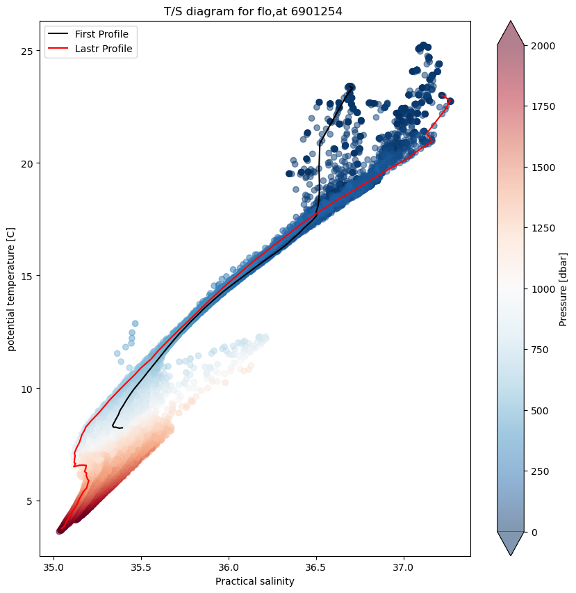
../../_images/a30f9e4608bc37a55dff3710adf7809f11d773894cb9cedd58b4b712162fb49c.png

TS-diagram#

In oceanography, temperature-salinity diagrams, sometimes called T-S diagrams, are used to identify water masses. In a T-S diagram, rather than plotting plotting temperatute and salinity as a separate “profile,” with pressure or depth as the vertical coordinate, potential temperature (on the vertical axis) is plotted versus salinity (on the horizontal axis).

This diagrams area very useful since as long as it remains isolated from the surface, where heat or fresh water can be gained or lost, and in the absence of mixing with other water masses, a water parcel’s potential temperature and salinity are conserved. Deep water masses thus retain their T-S characteristics for long periods of time, and can be identified readily on a T-S plot.

In this case we add a colobar bar to show the pressure of each data point.

import seawater as sw

/var/folders/tj/cj2twzcd30jbzn574lsp6phw0000gn/T/ipykernel_56518/1793873256.py:1: UserWarning: The seawater library is deprecated! Please use gsw instead.
  import seawater as sw

temp=prof.TEMP.values.flatten()
psal=prof.PSAL.values.flatten()
pres=prof.PRES.values.flatten()

compute potential temperature

ptmp=sw.ptmp(psal, temp, pres, pr=0)

fig, ax = plt.subplots(figsize=(10,10))
sc=ax.scatter(psal, ptmp, c=pres,alpha=0.5, cmap="RdBu_r",vmin=0, vmax=2000)
ax.set_title(f"T/S diagram for float {prof.PLATFORM_NUMBER[0].astype(str).values}")
ax.set_ylabel("potential temperature [C]")
ax.set_xlabel(f"{prof.PSAL.long_name}")
cbar=fig.colorbar(sc,extend='both');
cbar.set_label('Pressure [dbar]')

../../_images/8bbae2e546cf3332ee3b9cf11bca6d093d6588f5fdbff12c87d1df5805a418bb.png

Metadata#

And of course, all the metadata information for each profile is included in the netCDF file:

for i1 in range(1,prof.sizes['N_PROF'],10):
    print(f"Cycle {prof.data_vars['CYCLE_NUMBER'].values.astype(int)[i1]}"
          f" Direction {prof.data_vars['DIRECTION'].values.astype(str)[i1]}"
          f" WMO {prof.data_vars['PLATFORM_NUMBER'].values.astype(str)[i1]}"
          f" Data Center {prof.data_vars['DATA_CENTRE'].values.astype(str)[i1]}"   
          f" Project {prof.data_vars['PROJECT_NAME'].values.astype(str)[i1]}" )

Cycle 1 Direction A WMO 6901254  Data Center IF Project ARGO SPAIN                                                      
Cycle 11 Direction A WMO 6901254  Data Center IF Project ARGO SPAIN                                                      
Cycle 21 Direction A WMO 6901254  Data Center IF Project ARGO SPAIN                                                      
Cycle 31 Direction A WMO 6901254  Data Center IF Project ARGO SPAIN                                                      
Cycle 41 Direction A WMO 6901254  Data Center IF Project ARGO SPAIN                                                      
Cycle 51 Direction A WMO 6901254  Data Center IF Project ARGO SPAIN                                                      
Cycle 61 Direction A WMO 6901254  Data Center IF Project ARGO SPAIN                                                      
Cycle 71 Direction A WMO 6901254  Data Center IF Project ARGO SPAIN                                                      
Cycle 81 Direction A WMO 6901254  Data Center IF Project ARGO SPAIN                                                      
Cycle 91 Direction A WMO 6901254  Data Center IF Project ARGO SPAIN                                                      
Cycle 101 Direction A WMO 6901254  Data Center IF Project ARGO SPAIN                                                      

We can see the WMO number, the DAC (IF, for Ifremer) and the owner of the float: Argo Spain

Accessing all profiles at once

Contents

Accessing all profiles at once#

TS-diagram#

Metadata#