Within the folder for each float there is also a netCDF file with the data during the time the float was drifting, this is the data not included during the profiling part of the cycle.
Julian day (UTC) of each measurement relative to REFERENCE_DATE_TIME
standard_name :
time
conventions :
Relative julian days with decimal part (as parts of day)
resolution :
1.1574074074074073e-05
axis :
T
comment_on_resolution :
JULD resolution is 1 second, except for measurement codes [89 100 190 203 250 290 300 500 503 590 600 700 800] for which JULD resolution is 1 minute and for measurement codes [150 450 901] for which JULD resolution is 6 minutes
[6853 values with dtype=datetime64[ns]]
JULD_STATUS
(N_MEASUREMENT)
object
...
long_name :
Status of the date and time
conventions :
Argo reference table 19
[6853 values with dtype=object]
JULD_QC
(N_MEASUREMENT)
object
...
long_name :
Quality on date and time
conventions :
Argo reference table 2
[6853 values with dtype=object]
JULD_ADJUSTED
(N_MEASUREMENT)
datetime64[ns]
...
long_name :
Adjusted julian day (UTC) of each measurement relative to REFERENCE_DATE_TIME
standard_name :
time
conventions :
Relative julian days with decimal part (as parts of day)
resolution :
1.1574074074074073e-05
axis :
T
comment_on_resolution :
JULD_ADJUSTED resolution is 1 second, except for measurement codes [89 100 190 203 250 290 300 500 503 590 600 700 800] for which JULD_ADJUSTED resolution is 1 minute and for measurement codes [150 450 901] for which JULD_ADJUSTED resolution is 6 minutes
[6853 values with dtype=datetime64[ns]]
JULD_ADJUSTED_STATUS
(N_MEASUREMENT)
object
...
long_name :
Status of the JULD_ADJUSTED date
conventions :
Argo reference table 19
[6853 values with dtype=object]
JULD_ADJUSTED_QC
(N_MEASUREMENT)
object
...
long_name :
Quality on adjusted date and time
conventions :
Argo reference table 2
[6853 values with dtype=object]
LATITUDE
(N_MEASUREMENT)
float64
...
long_name :
Latitude of each location
standard_name :
latitude
units :
degree_north
valid_min :
-90.0
valid_max :
90.0
axis :
Y
[6853 values with dtype=float64]
LONGITUDE
(N_MEASUREMENT)
float64
...
long_name :
Longitude of each location
standard_name :
longitude
units :
degree_east
valid_min :
-180.0
valid_max :
180.0
axis :
X
[6853 values with dtype=float64]
POSITION_ACCURACY
(N_MEASUREMENT)
object
...
long_name :
Estimated accuracy in latitude and longitude
conventions :
Argo reference table 5
[6853 values with dtype=object]
POSITION_QC
(N_MEASUREMENT)
object
...
long_name :
Quality on position
conventions :
Argo reference table 2
[6853 values with dtype=object]
CYCLE_NUMBER
(N_MEASUREMENT)
float64
...
long_name :
Float cycle number of the measurement
conventions :
0...N, 0 : launch cycle, 1 : first complete cycle
[6853 values with dtype=float64]
CYCLE_NUMBER_ADJUSTED
(N_MEASUREMENT)
float64
...
long_name :
Adjusted float cycle number of the measurement
conventions :
0...N, 0 : launch cycle, 1 : first complete cycle
[6853 values with dtype=float64]
MEASUREMENT_CODE
(N_MEASUREMENT)
float64
...
long_name :
Flag referring to a measurement event in the cycle
conventions :
Argo reference table 15
[6853 values with dtype=float64]
AXES_ERROR_ELLIPSE_MAJOR
(N_MEASUREMENT)
float32
...
long_name :
Major axis of error ellipse from positioning system
units :
meters
[6853 values with dtype=float32]
AXES_ERROR_ELLIPSE_MINOR
(N_MEASUREMENT)
float32
...
long_name :
Minor axis of error ellipse from positioning system
units :
meters
[6853 values with dtype=float32]
AXES_ERROR_ELLIPSE_ANGLE
(N_MEASUREMENT)
float32
...
long_name :
Angle of error ellipse from positioning system
units :
Degrees (from North when heading East)
[6853 values with dtype=float32]
SATELLITE_NAME
(N_MEASUREMENT)
object
...
long_name :
Satellite name from positioning system
[6853 values with dtype=object]
PRES
(N_MEASUREMENT)
float32
...
long_name :
Sea water pressure, equals 0 at sea-level
standard_name :
sea_water_pressure
units :
decibar
valid_min :
0.0
valid_max :
12000.0
C_format :
%7.1f
FORTRAN_format :
F7.1
resolution :
1.0
comment_on_resolution :
PRES resolution is 1 dbar, except for measurement codes [150 198 398 497 498 901] for which PRES resolution is 10 dbar
axis :
Z
[6853 values with dtype=float32]
PRES_QC
(N_MEASUREMENT)
object
...
long_name :
quality flag
conventions :
Argo reference table 2
[6853 values with dtype=object]
PRES_ADJUSTED
(N_MEASUREMENT)
float32
...
long_name :
Sea water pressure, equals 0 at sea-level
standard_name :
sea_water_pressure
units :
decibar
valid_min :
0.0
valid_max :
12000.0
C_format :
%7.1f
FORTRAN_format :
F7.1
resolution :
1.0
comment_on_resolution :
PRES_ADJUSTED resolution is 1 dbar, except for measurement codes [150 198 398 497 498 901] for which PRES_ADJUSTED resolution is 10 dbar
axis :
Z
[6853 values with dtype=float32]
PRES_ADJUSTED_QC
(N_MEASUREMENT)
object
...
long_name :
quality flag
conventions :
Argo reference table 2
[6853 values with dtype=object]
PRES_ADJUSTED_ERROR
(N_MEASUREMENT)
float32
...
long_name :
Contains the error on the adjusted values as determined by the delayed mode QC process
units :
decibar
C_format :
%7.1f
FORTRAN_format :
F7.1
resolution :
1.0
[6853 values with dtype=float32]
TEMP
(N_MEASUREMENT)
float32
...
long_name :
Sea temperature in-situ ITS-90 scale
standard_name :
sea_water_temperature
units :
degree_Celsius
valid_min :
-2.5
valid_max :
40.0
C_format :
%9.3f
FORTRAN_format :
F9.3
resolution :
0.001
[6853 values with dtype=float32]
TEMP_QC
(N_MEASUREMENT)
object
...
long_name :
quality flag
conventions :
Argo reference table 2
[6853 values with dtype=object]
TEMP_ADJUSTED
(N_MEASUREMENT)
float32
...
long_name :
Sea temperature in-situ ITS-90 scale
standard_name :
sea_water_temperature
units :
degree_Celsius
valid_min :
-2.5
valid_max :
40.0
C_format :
%9.3f
FORTRAN_format :
F9.3
resolution :
0.001
[6853 values with dtype=float32]
TEMP_ADJUSTED_QC
(N_MEASUREMENT)
object
...
long_name :
quality flag
conventions :
Argo reference table 2
[6853 values with dtype=object]
TEMP_ADJUSTED_ERROR
(N_MEASUREMENT)
float32
...
long_name :
Contains the error on the adjusted values as determined by the delayed mode QC process
units :
degree_Celsius
C_format :
%9.3f
FORTRAN_format :
F9.3
resolution :
0.001
[6853 values with dtype=float32]
PSAL
(N_MEASUREMENT)
float32
...
long_name :
Practical salinity
standard_name :
sea_water_salinity
units :
psu
valid_min :
2.0
valid_max :
41.0
C_format :
%9.3f
FORTRAN_format :
F9.3
resolution :
0.001
[6853 values with dtype=float32]
PSAL_QC
(N_MEASUREMENT)
object
...
long_name :
quality flag
conventions :
Argo reference table 2
[6853 values with dtype=object]
PSAL_ADJUSTED
(N_MEASUREMENT)
float32
...
long_name :
Practical salinity
standard_name :
sea_water_salinity
units :
psu
valid_min :
2.0
valid_max :
41.0
C_format :
%9.3f
FORTRAN_format :
F9.3
resolution :
0.001
[6853 values with dtype=float32]
PSAL_ADJUSTED_QC
(N_MEASUREMENT)
object
...
long_name :
quality flag
conventions :
Argo reference table 2
[6853 values with dtype=object]
PSAL_ADJUSTED_ERROR
(N_MEASUREMENT)
float32
...
long_name :
Contains the error on the adjusted values as determined by the delayed mode QC process
units :
psu
C_format :
%9.3f
FORTRAN_format :
F9.3
resolution :
0.001
[6853 values with dtype=float32]
JULD_DESCENT_START
(N_CYCLE)
datetime64[ns]
...
long_name :
Descent start date of the cycle
standard_name :
time
conventions :
Relative julian days with decimal part (as parts of day)
resolution :
0.0006944444444444445
[103 values with dtype=datetime64[ns]]
JULD_DESCENT_START_STATUS
(N_CYCLE)
object
...
long_name :
Status of descent start date of the cycle
conventions :
Argo reference table 19
[103 values with dtype=object]
JULD_FIRST_STABILIZATION
(N_CYCLE)
datetime64[ns]
...
long_name :
Time when a float first becomes water-neutral
standard_name :
time
conventions :
Relative julian days with decimal part (as parts of day)
resolution :
0.004166666666666667
[103 values with dtype=datetime64[ns]]
JULD_FIRST_STABILIZATION_STATUS
(N_CYCLE)
object
...
long_name :
Status of time when a float first becomes water-neutral
conventions :
Argo reference table 19
[103 values with dtype=object]
JULD_DESCENT_END
(N_CYCLE)
datetime64[ns]
...
long_name :
Descent end date of the cycle
standard_name :
time
conventions :
Relative julian days with decimal part (as parts of day)
resolution :
0.0006944444444444445
[103 values with dtype=datetime64[ns]]
JULD_DESCENT_END_STATUS
(N_CYCLE)
object
...
long_name :
Status of descent end date of the cycle
conventions :
Argo reference table 19
[103 values with dtype=object]
JULD_PARK_START
(N_CYCLE)
datetime64[ns]
...
long_name :
Drift start date of the cycle
standard_name :
time
conventions :
Relative julian days with decimal part (as parts of day)
resolution :
0.0006944444444444445
[103 values with dtype=datetime64[ns]]
JULD_PARK_START_STATUS
(N_CYCLE)
object
...
long_name :
Status of drift start date of the cycle
conventions :
Argo reference table 19
[103 values with dtype=object]
JULD_PARK_END
(N_CYCLE)
datetime64[ns]
...
long_name :
Drift end date of the cycle
standard_name :
time
conventions :
Relative julian days with decimal part (as parts of day)
resolution :
0.0006944444444444445
[103 values with dtype=datetime64[ns]]
JULD_PARK_END_STATUS
(N_CYCLE)
object
...
long_name :
Status of drift end date of the cycle
conventions :
Argo reference table 19
[103 values with dtype=object]
JULD_DEEP_DESCENT_END
(N_CYCLE)
datetime64[ns]
...
long_name :
Deep descent end date of the cycle
standard_name :
time
conventions :
Relative julian days with decimal part (as parts of day)
resolution :
0.004166666666666667
[103 values with dtype=datetime64[ns]]
JULD_DEEP_DESCENT_END_STATUS
(N_CYCLE)
object
...
long_name :
Status of deep descent end date of the cycle
conventions :
Argo reference table 19
[103 values with dtype=object]
JULD_DEEP_PARK_START
(N_CYCLE)
datetime64[ns]
...
long_name :
Deep park start date of the cycle
standard_name :
time
conventions :
Relative julian days with decimal part (as parts of day)
resolution :
0.004166666666666667
[103 values with dtype=datetime64[ns]]
JULD_DEEP_PARK_START_STATUS
(N_CYCLE)
object
...
long_name :
Status of deep park start date of the cycle
conventions :
Argo reference table 19
[103 values with dtype=object]
JULD_ASCENT_START
(N_CYCLE)
datetime64[ns]
...
long_name :
Start date of the ascent to the surface
standard_name :
time
conventions :
Relative julian days with decimal part (as parts of day)
resolution :
0.0006944444444444445
[103 values with dtype=datetime64[ns]]
JULD_ASCENT_START_STATUS
(N_CYCLE)
object
...
long_name :
Status of start date of the ascent to the surface
conventions :
Argo reference table 19
[103 values with dtype=object]
JULD_DEEP_ASCENT_START
(N_CYCLE)
datetime64[ns]
...
long_name :
Deep ascent start date of the cycle
standard_name :
time
conventions :
Relative julian days with decimal part (as parts of day)
resolution :
0.0006944444444444445
[103 values with dtype=datetime64[ns]]
JULD_DEEP_ASCENT_START_STATUS
(N_CYCLE)
object
...
long_name :
Status of deep ascent start date of the cycle
conventions :
Argo reference table 19
[103 values with dtype=object]
JULD_ASCENT_END
(N_CYCLE)
datetime64[ns]
...
long_name :
End date of ascent to the surface
standard_name :
time
conventions :
Relative julian days with decimal part (as parts of day)
resolution :
0.0006944444444444445
[103 values with dtype=datetime64[ns]]
JULD_ASCENT_END_STATUS
(N_CYCLE)
object
...
long_name :
Status of end date of ascent to the surface
conventions :
Argo reference table 19
[103 values with dtype=object]
JULD_TRANSMISSION_START
(N_CYCLE)
datetime64[ns]
...
long_name :
Start date of transmission
standard_name :
time
conventions :
Relative julian days with decimal part (as parts of day)
resolution :
0.0006944444444444445
[103 values with dtype=datetime64[ns]]
JULD_TRANSMISSION_START_STATUS
(N_CYCLE)
object
...
long_name :
Status of start date of transmission
conventions :
Argo reference table 19
[103 values with dtype=object]
JULD_FIRST_MESSAGE
(N_CYCLE)
datetime64[ns]
...
long_name :
Date of earliest float message received
standard_name :
time
conventions :
Relative julian days with decimal part (as parts of day)
resolution :
1.1574074074074073e-05
[103 values with dtype=datetime64[ns]]
JULD_FIRST_MESSAGE_STATUS
(N_CYCLE)
object
...
long_name :
Status of date of earliest float message received
conventions :
Argo reference table 19
[103 values with dtype=object]
JULD_FIRST_LOCATION
(N_CYCLE)
datetime64[ns]
...
long_name :
Date of earliest location
standard_name :
time
conventions :
Relative julian days with decimal part (as parts of day)
resolution :
1.1574074074074073e-05
[103 values with dtype=datetime64[ns]]
JULD_FIRST_LOCATION_STATUS
(N_CYCLE)
object
...
long_name :
Status of date of earliest location
conventions :
Argo reference table 19
[103 values with dtype=object]
JULD_LAST_LOCATION
(N_CYCLE)
datetime64[ns]
...
long_name :
Date of latest location
standard_name :
time
conventions :
Relative julian days with decimal part (as parts of day)
resolution :
1.1574074074074073e-05
[103 values with dtype=datetime64[ns]]
JULD_LAST_LOCATION_STATUS
(N_CYCLE)
object
...
long_name :
Status of date of latest location
conventions :
Argo reference table 19
[103 values with dtype=object]
JULD_LAST_MESSAGE
(N_CYCLE)
datetime64[ns]
...
long_name :
Date of latest float message received
standard_name :
time
conventions :
Relative julian days with decimal part (as parts of day)
resolution :
1.1574074074074073e-05
[103 values with dtype=datetime64[ns]]
JULD_LAST_MESSAGE_STATUS
(N_CYCLE)
object
...
long_name :
Status of date of latest float message received
conventions :
Argo reference table 19
[103 values with dtype=object]
JULD_TRANSMISSION_END
(N_CYCLE)
datetime64[ns]
...
long_name :
Transmission end date
standard_name :
time
conventions :
Relative julian days with decimal part (as parts of day)
resolution :
0.0006944444444444445
[103 values with dtype=datetime64[ns]]
JULD_TRANSMISSION_END_STATUS
(N_CYCLE)
object
...
long_name :
Status of transmission end date
conventions :
Argo reference table 19
[103 values with dtype=object]
CLOCK_OFFSET
(N_CYCLE)
timedelta64[ns]
...
long_name :
Time of float clock drift
conventions :
Days with decimal part (as parts of day)
[103 values with dtype=timedelta64[ns]]
GROUNDED
(N_CYCLE)
object
...
long_name :
Did the profiler touch the ground for that cycle?
conventions :
Argo reference table 20
[103 values with dtype=object]
REPRESENTATIVE_PARK_PRESSURE
(N_CYCLE)
float32
...
long_name :
Best pressure value during park phase
units :
decibar
[103 values with dtype=float32]
REPRESENTATIVE_PARK_PRESSURE_STATUS
(N_CYCLE)
object
...
long_name :
Status of best pressure value during park phase
conventions :
Argo reference table 21
[103 values with dtype=object]
CONFIG_MISSION_NUMBER
(N_CYCLE)
float64
...
long_name :
Unique number denoting the missions performed by the float
conventions :
1...N, 1 : first complete mission
[103 values with dtype=float64]
CYCLE_NUMBER_INDEX
(N_CYCLE)
float64
...
long_name :
Cycle number that corresponds to the current index
conventions :
0...N, 0 : launch cycle, 1 : first complete cycle
[103 values with dtype=float64]
CYCLE_NUMBER_INDEX_ADJUSTED
(N_CYCLE)
float64
...
long_name :
Adjusted cycle number that corresponds to the current index
conventions :
0...N, 0 : launch cycle, 1 : first complete cycle
[103 values with dtype=float64]
DATA_MODE
(N_CYCLE)
object
...
long_name :
Delayed mode or real time data
conventions :
R : real time; D : delayed mode; A : real time with adjustment
[103 values with dtype=object]
HISTORY_INSTITUTION
(N_HISTORY)
object
...
long_name :
Institution which performed action
conventions :
Argo reference table 4
[1774 values with dtype=object]
HISTORY_STEP
(N_HISTORY)
object
...
long_name :
Step in data processing
conventions :
Argo reference table 12
[1774 values with dtype=object]
HISTORY_SOFTWARE
(N_HISTORY)
object
...
long_name :
Name of software which performed action
conventions :
Institution dependent
[1774 values with dtype=object]
HISTORY_SOFTWARE_RELEASE
(N_HISTORY)
object
...
long_name :
Version/release of software which performed action
conventions :
Institution dependent
[1774 values with dtype=object]
HISTORY_REFERENCE
(N_HISTORY)
object
...
long_name :
Reference of database
conventions :
Institution dependent
[1774 values with dtype=object]
HISTORY_DATE
(N_HISTORY)
object
...
long_name :
Date the history record was created
conventions :
YYYYMMDDHHMISS
[1774 values with dtype=object]
HISTORY_ACTION
(N_HISTORY)
object
...
long_name :
Action performed on data
conventions :
Argo reference table 7
[1774 values with dtype=object]
HISTORY_PARAMETER
(N_HISTORY)
object
...
long_name :
Station parameter action is performed on
conventions :
Argo reference table 3
[1774 values with dtype=object]
HISTORY_PREVIOUS_VALUE
(N_HISTORY)
float32
...
long_name :
Parameter/Flag previous value before action
[1774 values with dtype=float32]
HISTORY_INDEX_DIMENSION
(N_HISTORY)
object
...
long_name :
Name of dimension to which HISTORY_START_INDEX and HISTORY_STOP_INDEX correspond
conventions :
C: N_CYCLE, M: N_MEASUREMENT
[1774 values with dtype=object]
HISTORY_START_INDEX
(N_HISTORY)
float64
...
long_name :
Start index action applied on
[1774 values with dtype=float64]
HISTORY_STOP_INDEX
(N_HISTORY)
float64
...
long_name :
Stop index action applied on
[1774 values with dtype=float64]
HISTORY_QCTEST
(N_HISTORY)
object
...
long_name :
Documentation of tests performed, tests failed (in hex form)
conventions :
Write tests performed when ACTION=QCP$; tests failed when ACTION=QCF$
[1774 values with dtype=object]
title :
Argo float trajectory file
institution :
CORIOLIS
source :
Argo float
history :
2019-01-15T11:25:20Z creation; 2021-06-30T13:19:51Z last update (coriolis COQC software)
references :
http://www.argodatamgt.org/Documentation
user_manual_version :
3.1
Conventions :
Argo-3.1 CF-1.6
featureType :
trajectory
decoder_version :
CODA_043b
comment_on_resolution :
JULD and PRES variable resolutions depend on measurement codes
comment_on_measurement_code :
Meaning of some specific measurement codes for this float: 89: cycle start time, 190: descending profile dated levels, 198: max pressure sampled during descent to park pressure, 203: descending profile deepest level, 297: min pressure sampled during drift at park pressure, 298: max pressure sampled during drift at park pressure, 301: representative park measurement, 398: max pressure sampled during descent to profile pressure, 497: min pressure sampled during drift at profile pressure, 498: max pressure sampled during drift at profile pressure, 503: ascending profile deepest level, 590: ascending profile dated levels, 901: grounded information
once again the netCDF includes all the meta data to understand the data.
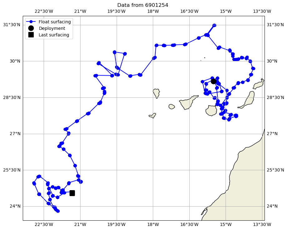
Let’s bgin by plotting the actual trayectory of the float.
importcartopy.crsasccrsimportcartopy
we use cartopy, so we can plot the coastile and the land:
lon=Rtraj.LONGITUDE[~np.isnan(Rtraj.LONGITUDE)&~np.isnan(Rtraj.LATITUDE)]lat=Rtraj.LATITUDE[~np.isnan(Rtraj.LONGITUDE)&~np.isnan(Rtraj.LATITUDE)]fig,ax=plt.subplots(figsize=(10,10),subplot_kw={'projection':ccrs.PlateCarree()})ax.plot(lon,lat,'-bo',label='Float surfacing')ax.plot(lon[0],lat[0],'ok',markersize=12,label='Deployment')ax.plot(lon[-1],lat[-1],'sk',markersize=12,label='Last surfacing')ax.add_feature(cartopy.feature.LAND.with_scale('10m'))ax.add_feature(cartopy.feature.COASTLINE.with_scale('10m'),edgecolor='black')ax.set_title(f"Data from {Rtraj.PLATFORM_NUMBER.values.astype(str)}")ax.legend()ax.gridlines(draw_labels=True,dms=True,x_inline=False,y_inline=False);
a blue dot for each time the float reached the surface.
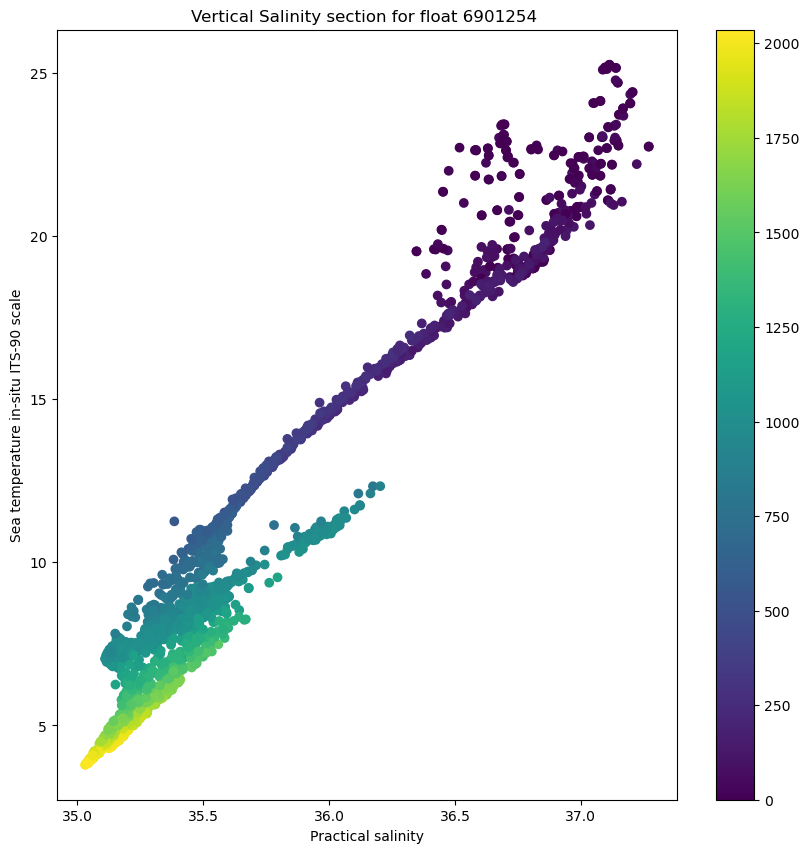
We can also plot the observations of Temperature and Salinity, in a TS diagram, during the drifting of the float:
fig,ax=plt.subplots(figsize=(10,10))sc=ax.scatter(Rtraj.PSAL,Rtraj.TEMP,c=Rtraj.PRES)ax.set_title(f"Vertical Salinity section for float {Rtraj.PLATFORM_NUMBER.astype(str).values}")ax.set_xlabel(f"{Rtraj.PSAL.long_name}")ax.set_ylabel(f"{Rtraj.TEMP.long_name}")fig.colorbar(sc);
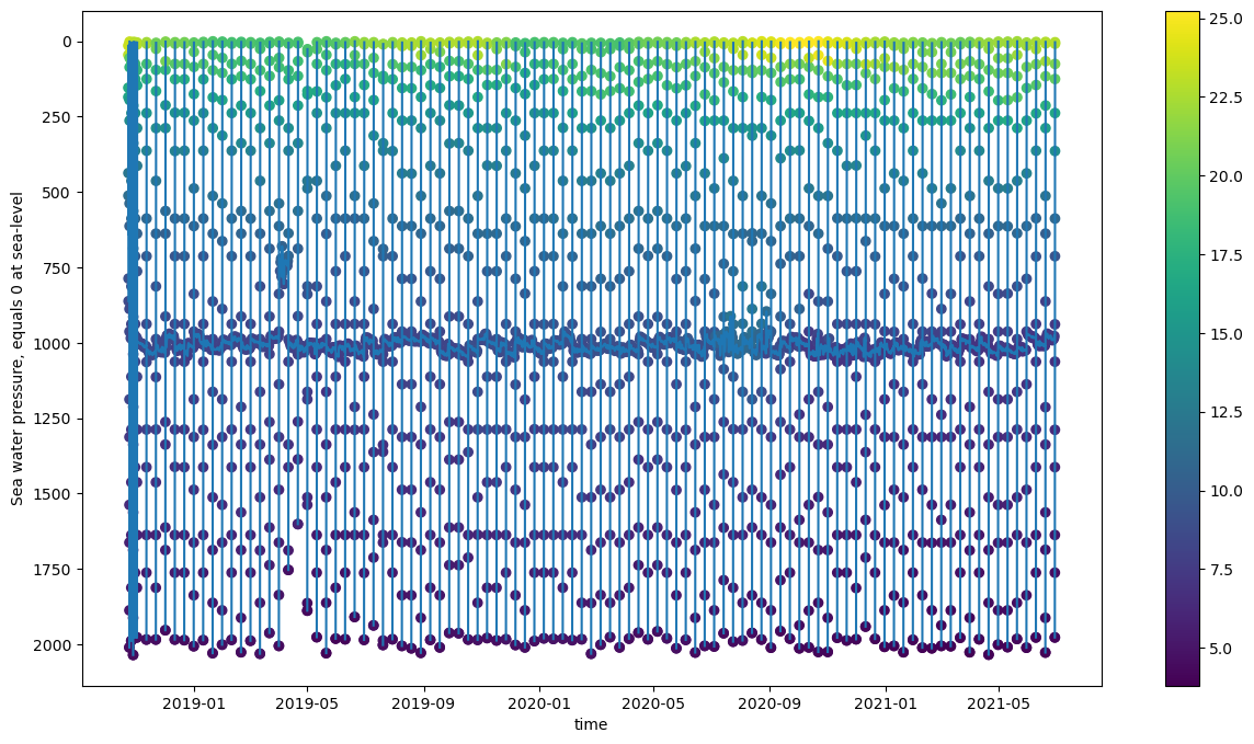
and the time-series of temperature, where we can see that most of the observations are at the parking depth,
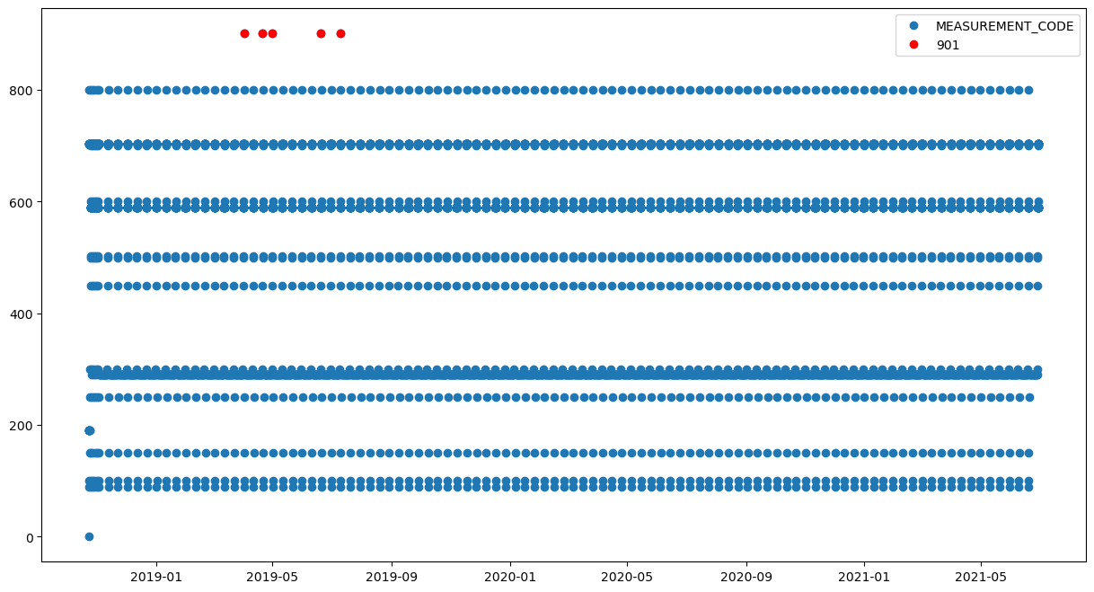
And we can see what observations we have in eacj data point, using the MEASUREMENT_CODE. As indicated in the Ago referente Table 15 of the Argo user’s manual, we have a few observations with code 901, that correspond to “Grounded flag Configuration phas”, in red in the follo