
Reading Argo data by date#
Let’s use, as an example, data in the *Atlantic for the 11th November 2020. It is pre-downloaded in the ./Data folder, but you can download it from the Coriolis GDAC See here for instructions on how to download the data
import numpy as np
import netCDF4
import xarray as xr

import cartopy.crs as ccrs
import cartopy

import matplotlib as mpl
import matplotlib.cm as cm
from matplotlib import pyplot as plt
%matplotlib inline
# Usefull colormaps and colorbar makers:
qcmap = mpl.colors.ListedColormap(['#000000' , '#31FC03' , '#ADFC03' , '#FCBA03' ,'#FC1C03',
                                   '#324CA8' , '#000000' , '#000000' , '#B22CC9', '#000000'])
def colorbar_qc(cmap, **kwargs):
    """Adjust colorbar ticks with discrete colors for QC flags"""
    ncolors = 10
    mappable = cm.ScalarMappable(cmap=cmap)
    mappable.set_array([])
    mappable.set_clim(-0.5, ncolors+0.5)
    colorbar = plt.colorbar(mappable, **kwargs)
    colorbar.set_ticks(np.linspace(0, ncolors, ncolors))
    colorbar.set_ticklabels(range(ncolors))
    return colorbar
dayADS = xr.open_dataset('../../Data/atlantic_ocean/2020/11/20201111_prof.nc')
dayADS
<xarray.Dataset>
Dimensions:                       (N_PROF: 188, N_PARAM: 3, N_LEVELS: 1331, N_CALIB: 3, N_HISTORY: 0)
Dimensions without coordinates: N_PROF, N_PARAM, N_LEVELS, N_CALIB, N_HISTORY
Data variables: (12/64)
    DATA_TYPE                     object b'Argo profile    '
    FORMAT_VERSION                object b'3.1 '
    HANDBOOK_VERSION              object b'1.2 '
    REFERENCE_DATE_TIME           object b'19500101000000'
    DATE_CREATION                 object b'20201111082709'
    DATE_UPDATE                   object b'20211211022000'
    ...                            ...
    HISTORY_ACTION                (N_HISTORY, N_PROF) object
    HISTORY_PARAMETER             (N_HISTORY, N_PROF) object
    HISTORY_START_PRES            (N_HISTORY, N_PROF) float32
    HISTORY_STOP_PRES             (N_HISTORY, N_PROF) float32
    HISTORY_PREVIOUS_VALUE        (N_HISTORY, N_PROF) float32
    HISTORY_QCTEST                (N_HISTORY, N_PROF) object
Attributes:
    title:                Argo float vertical profile
    institution:          FR GDAC
    source:               Argo float
    history:              2021-12-11T02:20:00Z creation
    references:           http://www.argodatamgt.org/Documentation
    user_manual_version:  3.1
    Conventions:          Argo-3.1 CF-1.6
featureType: trajectoryProfile- N_PROF: 188
- N_PARAM: 3
- N_LEVELS: 1331
- N_CALIB: 3
- N_HISTORY: 0
- DATA_TYPE()object...
- long_name :
- Data type
- conventions :
- Argo reference table 1
array(b'Argo profile ', dtype=object)
- FORMAT_VERSION()object...
- long_name :
- File format version
array(b'3.1 ', dtype=object)
- HANDBOOK_VERSION()object...
- long_name :
- Data handbook version
array(b'1.2 ', dtype=object)
- REFERENCE_DATE_TIME()object...
- long_name :
- Date of reference for Julian days
- conventions :
- YYYYMMDDHHMISS
array(b'19500101000000', dtype=object)
- DATE_CREATION()object...
- long_name :
- Date of file creation
- conventions :
- YYYYMMDDHHMISS
array(b'20201111082709', dtype=object)
- DATE_UPDATE()object...
- long_name :
- Date of update of this file
- conventions :
- YYYYMMDDHHMISS
array(b'20211211022000', dtype=object)
- PLATFORM_NUMBER(N_PROF)object...
- long_name :
- Float unique identifier
- conventions :
- WMO float identifier : A9IIIII
array([b'3901238 ', b'4903277 ', b'6903030 ', b'5904669 ', b'3901819 ', b'5905132 ', b'5902338 ', b'6902976 ', b'6903698 ', b'6903032 ', b'4902909 ', b'7900506 ', b'6903034 ', b'6903788 ', b'4903035 ', b'4902920 ', b'6903270 ', b'6902655 ', b'3902107 ', b'3901938 ', b'1901814 ', b'6901986 ', b'1902070 ', b'3901969 ', b'6901985 ', b'6901144 ', b'4903259 ', b'3902399 ', b'3901043 ', b'6903268 ', b'6903788 ', b'4902117 ', b'3901312 ', b'4903228 ', b'4903261 ', b'5905380 ', b'4903245 ', b'6902762 ', b'4902348 ', b'6902834 ', b'3901971 ', b'4902354 ', b'4902323 ', b'3902148 ', b'6903788 ', b'3902121 ', b'6901935 ', b'3901870 ', b'6901934 ', b'4902116 ', b'3902238 ', b'3901551 ', b'3902121 ', b'5904847 ', b'6901194 ', b'5905383 ', b'4903260 ', b'1902228 ', b'4901628 ', b'3901822 ', b'6903016 ', b'6902727 ', b'6903788 ', b'3902237 ', b'3901850 ', b'6902851 ', b'6902855 ', b'6902854 ', b'6902852 ', b'6902929 ', b'7900559 ', b'3901869 ', b'3901859 ', b'6902899 ', b'3901878 ', b'3901857 ', b'3901838 ', b'3902168 ', b'4902912 ', b'6903550 ', b'3901111 ', b'6902818 ', b'5906005 ', b'4902921 ', b'3902106 ', b'6901774 ', b'3902137 ', b'6903567 ', b'6903705 ', b'3902106 ', b'4903240 ', b'4903276 ', b'3902207 ', b'3901541 ', b'6902898 ', b'3902137 ', b'5905148 ', b'6903788 ', b'6901932 ', b'5905381 ', b'7900207 ', b'3901823 ', b'4902350 ', b'3901658 ', b'7900563 ', b'6903554 ', b'4903225 ', b'3901605 ', b'4902424 ', b'1902063 ', b'4901699 ', b'6903552 ', b'4903237 ', b'4902916 ', b'6901925 ', b'3902109 ', b'6902974 ', b'6902686 ', b'6901604 ', b'6901763 ', b'4902456 ', b'3901633 ', b'3902110 ', b'6902837 ', b'3901526 ', b'3901540 ', b'3901644 ', b'1901712 ', b'3902109 ', b'6903558 ', b'3902208 ', b'6902944 ', b'6903266 ', b'6901281 ', b'6903788 ', b'3902110 ', b'3901977 ', b'6903786 ', b'3901867 ', b'7900596 ', b'6900893 ', b'6900892 ', b'4902455 ', b'6903255 ', b'7900516 ', b'7900534 ', b'6901266 ', b'3901675 ', b'7900542 ', b'6902870 ', b'3901673 ', b'6901254 ', b'6902873 ', b'7900524 ', b'6901255 ', b'5906215 ', b'6902875 ', b'4902523 ', b'3901937 ', b'3901622 ', b'4902524 ', b'4902505 ', b'5905076 ', b'4902509 ', b'6901278 ', b'4902501 ', b'6901208 ', b'1901819 ', b'4902510 ', b'4901702 ', b'4902471 ', b'3901601 ', b'3901931 ', b'1901822 ', b'6903723 ', b'6903788 ', b'3901226 ', b'4902345 ', b'3901983 ', b'6902964 ', b'6903273 ', b'6902965 ', b'4901625 ', b'4903236 ', b'5903661 ', b'4902346 ', b'6901726 ', b'6903788 '], dtype=object) - PROJECT_NAME(N_PROF)object...
- long_name :
- Name of the project
array([b'US ARGO PROJECT ', b'US ARGO PROJECT ', b'OVIDE ', b'UW, Argo ', b'US ARGO PROJECT ', b'UW, SOCCOM, Argo equivalent ', b'Argo ', b'OVIDE ', b'ARGO-FINLAND ', b'OVIDE ', b'US ARGO PROJECT ', b'ARGO-BSH ', b'OVIDE ', b'Argo Italy ', b'US ARGO PROJECT ', b'US ARGO PROJECT ', b'ARGO Italy ', b'Coriolis ', b'ARGO POLAND ', b'MOCCA-EU ', b'US ARGO PROJECT ', b'Argo Netherlands ', b'US ARGO PROJECT ', b'MOCCA-NETH ', b'Argo Netherlands ', b'Argo UK ', b'US ARGO PROJECT ', b'Argo UK ', b'US ARGO PROJECT ', b'Argo-Italy ', b'Argo Italy ', b'US ARGO PROJECT ', b'US ARGO PROJECT ', b'US ARGO PROJECT ', b'US ARGO PROJECT ', b'UW, Argo ', b'US ARGO PROJECT ', b'PIRATA ', b'US ARGO PROJECT ', b'CORIOLIS ', b'MOCCA-EU ', b'US ARGO PROJECT ', b'US ARGO PROJECT ', b'US ARGO PROJECT ', b'Argo Italy ', b'AtlantOS ', b'ARGO_IRELAND ', b'MOCCA-EU ', b'Argo Ireland ', b'US ARGO PROJECT ', b'US ARGO PROJECT ', b'Argo UK ', b'AtlantOS ', b'UW, SOCCOM, Argo equivalent ', b'Argo UK ', b'UW, Argo ', b'US ARGO PROJECT ', b'US ARGO PROJECT ', b'US ARGO PROJECT ', b'US ARGO PROJECT ', b'CORIOLIS ', b'CORIOLIS ', b'Argo Italy ', b'US ARGO PROJECT ', b'MOCCA-POLAND ', b'GMMC ARGOMEX ', b'GMMC ARGOMEX ', b'GMMC ARGOMEX ', b'GMMC ARGOMEX ', b'PIRATA ', b'Argo GERMANY ', b'MOCCA-EU ', b'MOCCA-EU ', b'Euro-Argo RISE ', b'MOCCA-NETH ', b'MOCCA-EU ', b'MOCCA-GER ', b'US ARGO PROJECT ', b'US ARGO PROJECT ', b'Norway-BGC-Argo ', b'US ARGO PROJECT ', b'GMMC OVIDE ', b'UW, SOCCOM, Argo equivalent ', b'US ARGO PROJECT ', b'ARGO POLAND ', b'NAOS ', b'MOCCA-EU ', b'Argo-Norway ', b'Argo-Finland ', b'ARGO POLAND ', b'US ARGO PROJECT ', b'US ARGO PROJECT ', b'US ARGO PROJECT ', b'Argo UK ', b'NAOS ', b'MOCCA-EU ', b'UW, Argo ', b'Argo Italy ', b'Argo Ireland ', b'UW, Argo ', b'US ARGO PROJECT ', b'US ARGO PROJECT ', b'US ARGO PROJECT ', b'ARGO-BSH ', b'Argo GERMANY ', b'ARGO Norway ', b'US ARGO PROJECT ', b'ARGO-BSH ', b'Argo Canada ', b'US ARGO PROJECT ', b'US ARGO PROJECT ', b'Argo-Norway ', b'US ARGO PROJECT ', b'US ARGO PROJECT ', b'Argo Ireland ', b'Euro-Argo RISE ', b'OVIDE ', b'RREX ', b'OVIDE ', b'GMMC OVIDE ', b'Argo Canada ', b'ARGO-BSH ', b'ARGO POLAND ', b'CORIOLIS ', b'Argo UK ', b'Argo UK ', b'ARGO-BSH ', b'US ARGO PROJECT ', b'Euro-Argo RISE ', b'Norway-BGC-Argo ', b'US ARGO PROJECT ', b'PERLE ', b'Argo Italy,CALYPSO 2019 ', b'ARGO SPAIN ', b'Argo Italy ', b'ARGO POLAND ', b'ARGO Italy ', b'Argo Italy ', b'MOCCA-EU ', b'ARGO Bulgary ', b'ARGO-BSH ', b'ARGO-BSH ', b'Argo Canada ', b'ARGO Italy ', b'ARGO-BSH ', b'ARGO-BSH ', b'ARGO SPAIN ', b'ARGO-BSH ', b'ARGO-BSH ', b'GMMC PERLE ', b'ARGO-BSH ', b'ARGO SPAIN ', b'GMMC PERLE ', b'ARGO-BSH ', b'ARGO SPAIN ', b'UW, SOCCOM, Argo equivalent ', b'GMMC PERLE ', b'Argo Canada ', b'MOCCA-EU ', b'ARGO-BSH ', b'Argo Canada ', b'Argo Canada ', b'UW, SOCCOM, Argo equivalent ', b'Argo Canada ', b'Euro-Argo RISE ', b'Argo Canada ', b'Argo UK ', b'US ARGO PROJECT ', b'Argo Canada ', b'US ARGO PROJECT ', b'Argo Canada ', b'ARGO-BSH ', b'MOCCA-EU ', b'US ARGO PROJECT ', b'Argo UK ', b'Argo Italy ', b'US ARGO PROJECT ', b'US ARGO PROJECT ', b'MOCCA-EU ', b'CORIOLIS ', b'ARGO Norway ', b'MOOSE ', b'US ARGO PROJECT ', b'US ARGO PROJECT ', b'Argo Australia ', b'US ARGO PROJECT ', b'RREX ASFAR ', b'Argo Italy '], dtype=object) - PI_NAME(N_PROF)object...
- long_name :
- Name of the principal investigator
array([b'BRECK OWENS, STEVEN JAYNE, P.E. ROBBINS ', b'WHOI: WIJFFELS, JAYNE, ROBBINS ', b'Damien DESBRUYERES ', b'STEPHEN RISER ', b'BRECK OWENS, STEVEN JAYNE, P.E. ROBBINS ', b'STEPHEN RISER, KENNETH JOHNSON ', b'DEAN ROEMMICH ', b'Damien DESBRUYERES ', b'Laura Tuomi ', b'Damien DESBRUYERES ', b'BRECK OWENS, STEVEN JAYNE, P.E. ROBBINS ', b'Birgit KLEIN ', b'Damien DESBRUYERES ', b'Pierre-Marie Poulain ', b'BRECK OWENS, STEVEN JAYNE, P.E. ROBBINS ', b'BRECK OWENS, STEVEN JAYNE, P.E. ROBBINS ', b'Pierre-Marie Poulain ', b'Christine COATANOAN ', b'Waldemar Walczowski ', b'Romain Cancouet ', b'BRECK OWENS, STEVEN JAYNE, P.E. ROBBINS ', b'Andreas Sterl ', b'BRECK OWENS, STEVEN JAYNE, P.E. ROBBINS ', b'Andreas Sterl ', b'Andreas Sterl ', b'Jon Turton ', b'AMY BOWER, STEVEN JAYNE, HEATHER FUREY ', b'Jon Turton ', b'BRECK OWENS, STEVE JAYNE, P.E. ROBBINS ', b'Pierre-Marie Poulain ', b'Pierre-Marie Poulain ', b'BRECK OWENS, STEVEN JAYNE, P.E. ROBBINS ', b'GREGORY C. JOHNSON ', b'WHOI: WIJFFELS, JAYNE, ROBBINS ', b'WHOI: WIJFFELS, JAYNE, ROBBINS ', b'STEPHEN RISER, ', b'WIJFFELS, JAYNCE, ROBBINS ', b'Bernard BOURLES ', b'BRECK OWENS, STEVEN JAYNE, P.E. ROBBINS ', b'Christine COATANOAN ', b'Romain Cancouet ', b'BRECK OWENS, STEVEN JAYNE, P.E. ROBBINS ', b'DEAN ROEMMICH ', b'GREGORY C. JOHNSON ', b'Pierre-Marie Poulain ', b'Herve CLAUSTRE ', b"Conall O'Malley ", b'Peter Brandt ', b"Conall O'Malley ", b'BRECK OWENS, STEVEN JAYNE, P.E. ROBBINS ', b'WHOI: WIJFFELS, JAYNE, ROBBINS ', b'Jon Turton ', b'Herve CLAUSTRE ', b'STEPHEN RISER, KENNETH JOHNSON ', b'Jon Turton ', b'STEPHEN RISER, ', b'WHOI: WIJFFELS, JAYNE, ROBBINS ', b'WHOI: WIJFFELS, JAYNE, ROBBINS ', b'BRECK OWENS, STEVEN JAYNE, P.E. ROBBINS ', b'BRECK OWENS, STEVEN JAYNE, P.E. ROBBINS ', b'Franck DUMAS ', b'Marcel BABIN ', b'Pierre-Marie Poulain ', b'WIJFFELS, JAYNE, ROBBINS ', b'Waldemar Walczowski ', b"Fabrizio D'ORTENZIO ", b"Fabrizio D'ORTENZIO ", b"Fabrizio D'ORTENZIO ", b"Fabrizio D'ORTENZIO ", b'Bernard BOURLES ', b'Oliver Zielinski ', b'Peter Brandt ', b'Romain Cancouet ', b"Fabrizio D'ORTENZIO ", b'Andreas Sterl ', b'Romain Cancouet ', b'Birgit Klein ', b'WIJFFELS, JAYNE, ROBBINS ', b'BRECK OWENS, STEVEN JAYNE, P.E. ROBBINS ', b'Kjell Arne Mork ', b'BRECK OWENS, STEVEN JAYNE, P.E. ROBBINS ', b'Virginie THIERRY ', b'STEPHEN RISER, KENNETH JOHNSON ', b'BRECK OWENS, STEVEN JAYNE, P.E. ROBBINS ', b'Waldemar Walczowski ', b"Fabrizio D'ORTENZIO ", b'Romain Cancouet ', b'Kjell Arne Mork ', b'J. Haapala ', b'Waldemar Walczowski ', b'AMY BOWER, STEVEN JAYNE, HEATHER FUREY ', b'WHOI: WIJFFELS, JAYNE, ROBBINS ', b'GREGORY C. JOHNSON ', b'Brian King ', b"Fabrizio D'ORTENZIO ", b'Romain Cancouet ', b'STEPHEN RISER ', b'Pierre-Marie Poulain ', b"Diarmuid O'Conchubhair ", b'STEPHEN RISER, ', b'DEAN ROEMMICH ', b'BRECK OWENS, STEVEN JAYNE, P.E. ROBBINS ', b'BRECK OWENS, STEVEN JAYNE, P.E. ROBBINS ', b'Birgit Klein ', b'Oliver Zielinski ', b'Kjell Arne Mork ', b'WHOI: WIJFFELS, JAYNE, ROBBINS ', b'Birgit KLEIN ', b'Blair Greenan ', b'BRECK OWENS, STEVEN JAYNE, P.E. ROBBINS ', b'BRECK OWENS, STEVEN JAYNE, P.E. ROBBINS ', b'Kjell Arne Mork ', b'AMY BOWER, STEVEN JAYNE, HEATHER FUREY ', b'BRECK OWENS, STEVEN JAYNE, P.E. ROBBINS ', b"Diarmuid O'Conchubhair ", b'Waldemar Walczowski ', b'Damien DESBRUYERES ', b'Virginie THIERRY ', b'Damien DESBRUYERES ', b'Virginie THIERRY ', b'Blair Greenan ', b'Birgit Klein ', b'Waldemar Walczowski ', b'Christine COATANOAN ', b'Jon Turton ', b'Brian King ', b'Birgit Klein ', b'BRECK OWENS, STEVE JAYNE, P.E. ROBBINS ', b'Waldemar Walczowski ', b'Kjell Arne Mork ', b'GREGORY C. JOHNSON ', b'Franck DUMAS ', b'Pierre-Marie Poulain ', b'Inmaculada Ruiz-Parrado ', b'Pierre-Marie Poulain ', b'Waldemar Walczowski ', b'Pierre-Marie Poulain ', b'Pierre-Marie Poulain ', b'Peter Brandt ', b'Violeta SLABAKOVA ', b'Birgit Klein ', b'Birgit Klein ', b'Blair Greenan ', b'Pierre-Marie Poulain ', b'Birgit Klein ', b'Birgit Klein ', b'Pedro Velez ', b'Birgit Klein ', b'Dr. Birgit Klein ', b'Laurent COPPOLA ', b'Birgit Klein ', b'Pedro Velez ', b'Laurent COPPOLA ', b'Birgit Klein ', b'Pedro Velez ', b'STEPHEN RISER, KENNETH JOHNSON ', b'Laurent COPPOLA ', b'Blair Greenan ', b'Sabrina Speich ', b'Birgit Klein ', b'Blair Greenan ', b'Blair Greenan ', b'STEPHEN RISER, KENNETH JOHNSON ', b'Blair Greenan ', b'Inmaculada Ruiz-Parrado ', b'Blair Greenan ', b'Jon Turton ', b'BRECK OWENS, STEVEN JAYNE, P.E. ROBBINS ', b'Blair Greenan ', b'BRECK OWENS, STEVEN JAYNE, P.E. ROBBINS ', b'Blair Greenan ', b'Birgit KLEIN ', b'Sabrina Speich ', b'BRECK OWENS, STEVEN JAYNE, P.E. ROBBINS ', b'Jon Turton ', b'Pierre-Marie Poulain ', b'BRECK OWENS, STEVEN JAYNE, P.E. ROBBINS ', b'BRECK OWENS, STEVEN JAYNE, P.E. ROBBINS ', b'Josep Lluis Pelegri ', b'Sabrina SPEICH ', b'Kjell Arne MORK ', b'Laurent COPPOLA ', b'BRECK OWENS, STEVEN JAYNE, P.E. ROBBINS ', b'AMY BOWER, STEVEN JAYNE, HEATHER FUREY ', b'Susan Wijffels ', b'BRECK OWENS, STEVEN JAYNE, P.E. ROBBINS ', b'Virginie THIERRY ', b'Pierre-Marie Poulain '], dtype=object) - STATION_PARAMETERS(N_PROF, N_PARAM)object...
- long_name :
- List of available parameters for the station
- conventions :
- Argo reference table 3
array([[b'PRES ', b'TEMP ', b'PSAL '], [b'PRES ', b'TEMP ', b'PSAL '], [b'PRES ', b'TEMP ', b'PSAL '], ..., [b'PRES ', b'TEMP ', b'PSAL '], [b'PRES ', b'TEMP ', b'PSAL '], [b'PRES ', b'TEMP ', b'PSAL ']], dtype=object) - CYCLE_NUMBER(N_PROF)float64...
- long_name :
- Float cycle number
- conventions :
- 0...N, 0 : launch cycle (if exists), 1 : first complete cycle
array([140., 10., 9., 180., 248., 113., 281., 9., 272., 9., 130., 138., 9., 110., 117., 116., 86., 181., 93., 114., 148., 39., 114., 95., 38., 293., 85., 38., 260., 78., 109., 163., 54., 29., 29., 103., 47., 133., 160., 80., 85., 241., 101., 49., 108., 266., 7., 147., 8., 163., 41., 76., 265., 69., 157., 103., 38., 40., 247., 130., 27., 175., 107., 46., 161., 165., 165., 165., 165., 151., 168., 147., 154., 114., 131., 156., 155., 48., 253., 110., 194., 87., 62., 116., 407., 146., 401., 37., 22., 406., 102., 10., 47., 141., 246., 400., 114., 106., 54., 103., 216., 248., 153., 103., 31., 120., 32., 152., 92., 147., 238., 4., 102., 250., 172., 238., 13., 121., 13., 88., 77., 114., 85., 68., 149., 141., 69., 307., 237., 54., 33., 240., 263., 2., 105., 84., 151., 12., 150., 35., 41., 40., 77., 63., 69., 53., 89., 89., 36., 128., 90., 79., 136., 54., 60., 31., 128., 4., 141., 118., 4., 11., 136., 11., 100., 4., 86., 165., 11., 239., 52., 152., 140., 148., 2., 104., 194., 159., 116., 109., 196., 13., 246., 103., 357., 162., 158., 103.]) - DIRECTION(N_PROF)object...
- long_name :
- Direction of the station profiles
- conventions :
- A: ascending profiles, D: descending profiles
array([b'A', b'A', b'A', b'A', b'A', b'A', b'A', b'A', b'A', b'A', b'A', b'A', b'A', b'A', b'A', b'A', b'A', b'A', b'A', b'A', b'A', b'A', b'A', b'A', b'A', b'A', b'A', b'A', b'A', b'A', b'A', b'A', b'D', b'A', b'A', b'A', b'A', b'A', b'A', b'A', b'A', b'A', b'D', b'D', b'A', b'D', b'A', b'A', b'A', b'A', b'A', b'A', b'A', b'A', b'A', b'A', b'A', b'A', b'A', b'A', b'A', b'A', b'A', b'A', b'A', b'A', b'A', b'A', b'A', b'A', b'A', b'A', b'A', b'A', b'A', b'A', b'A', b'A', b'A', b'A', b'A', b'A', b'A', b'A', b'D', b'A', b'D', b'A', b'A', b'A', b'A', b'A', b'D', b'A', b'A', b'A', b'A', b'A', b'A', b'A', b'A', b'A', b'A', b'A', b'A', b'A', b'A', b'A', b'A', b'A', b'A', b'A', b'A', b'A', b'A', b'D', b'A', b'A', b'A', b'A', b'A', b'A', b'D', b'A', b'A', b'A', b'A', b'A', b'A', b'A', b'A', b'A', b'A', b'A', b'A', b'A', b'A', b'A', b'A', b'A', b'A', b'A', b'A', b'A', b'A', b'A', b'A', b'A', b'A', b'A', b'A', b'A', b'A', b'A', b'A', b'A', b'A', b'A', b'A', b'A', b'A', b'A', b'A', b'A', b'A', b'A', b'A', b'A', b'A', b'A', b'A', b'A', b'A', b'A', b'A', b'A', b'A', b'A', b'A', b'A', b'A', b'A', b'A', b'A', b'A', b'A', b'A', b'A'], dtype=object) - DATA_CENTRE(N_PROF)object...
- long_name :
- Data centre in charge of float data processing
- conventions :
- Argo reference table 4
array([b'AO', b'AO', b'IF', b'AO', b'AO', b'AO', b'AO', b'IF', b'IF', b'IF', b'AO', b'IF', b'IF', b'IF', b'AO', b'AO', b'IF', b'IF', b'IF', b'BO', b'AO', b'IF', b'AO', b'BO', b'IF', b'BO', b'AO', b'BO', b'AO', b'IF', b'IF', b'AO', b'AO', b'AO', b'AO', b'AO', b'AO', b'IF', b'AO', b'IF', b'BO', b'AO', b'AO', b'AO', b'IF', b'IF', b'BO', b'IF', b'BO', b'AO', b'AO', b'BO', b'IF', b'AO', b'BO', b'AO', b'AO', b'AO', b'AO', b'AO', b'IF', b'IF', b'IF', b'AO', b'IF', b'IF', b'IF', b'IF', b'IF', b'IF', b'IF', b'IF', b'IF', b'IF', b'BO', b'IF', b'IF', b'AO', b'AO', b'IF', b'AO', b'IF', b'AO', b'AO', b'IF', b'IF', b'IF', b'IF', b'IF', b'IF', b'AO', b'AO', b'AO', b'BO', b'IF', b'IF', b'AO', b'IF', b'BO', b'AO', b'AO', b'AO', b'AO', b'IF', b'IF', b'IF', b'AO', b'IF', b'ME', b'AO', b'AO', b'IF', b'AO', b'AO', b'BO', b'IF', b'IF', b'IF', b'IF', b'IF', b'ME', b'IF', b'IF', b'IF', b'BO', b'BO', b'IF', b'AO', b'IF', b'IF', b'AO', b'IF', b'IF', b'IF', b'IF', b'IF', b'IF', b'IF', b'IF', b'IF', b'IF', b'IF', b'ME', b'IF', b'IF', b'IF', b'IF', b'IF', b'IF', b'IF', b'IF', b'IF', b'IF', b'IF', b'IF', b'AO', b'IF', b'ME', b'IF', b'IF', b'ME', b'ME', b'AO', b'ME', b'IF', b'ME', b'BO', b'AO', b'ME', b'AO', b'ME', b'IF', b'IF', b'AO', b'BO', b'IF', b'AO', b'AO', b'BO', b'IF', b'IF', b'IF', b'AO', b'AO', b'CS', b'AO', b'IF', b'IF'], dtype=object) - DC_REFERENCE(N_PROF)object...
- long_name :
- Station unique identifier in data centre
- conventions :
- Data centre convention
array([b'7104 ', b'8480 ', b' ', b'6179 ', b'7133 ', b'7073 ', b'5166 ', b' ', b' ', b' ', b'7111 ', b' ', b' ', b' ', b'7490 ', b'7472 ', b' ', b' ', b' ', b' ', b'6481 ', b' ', b'7477 ', b' ', b' ', b'137170 ', b'8047 ', b'137166 ', b'5136 ', b' ', b' ', b'6730 ', b'7940 ', b'8003 ', b'8458 ', b'7441 ', b'8020 ', b' ', b'6747 ', b' ', b' ', b'7109 ', b'6848 ', b'7943 ', b' ', b' ', b' ', b' ', b' ', b'6729 ', b'8030 ', b'137164 ', b' ', b'6704 ', b'137158 ', b'7444 ', b'8053 ', b'8034 ', b'5359 ', b'7136 ', b' ', b' ', b' ', b'8029 ', b' ', b' ', b' ', b' ', b' ', b' ', b' ', b' ', b' ', b' ', b' ', b' ', b' ', b'8025 ', b'7114 ', b' ', b'6440 ', b' ', b'7688 ', b'7473 ', b' ', b' ', b' ', b' ', b' ', b' ', b'8015 ', b'8479 ', b'7966 ', b'138577 ', b' ', b' ', b'7089 ', b' ', b' ', b'7442 ', b'5606_008321_216 ', b'7137 ', b'6749 ', b' ', b' ', b' ', b'8000 ', b' ', b'4902424_9931_TE ', b'7094 ', b'5491 ', b' ', b'8012 ', b'7130 ', b'137152 ', b' ', b' ', b' ', b' ', b' ', b'4902456_9930_TE ', b' ', b' ', b' ', b'137159 ', b'138569 ', b' ', b'5343 ', b' ', b' ', b'7975 ', b' ', b' ', b' ', b' ', b' ', b' ', b' ', b' ', b' ', b' ', b' ', b'4902455_9926_TE ', b' ', b' ', b' ', b' ', b' ', b' ', b' ', b' ', b' ', b' ', b' ', b' ', b'8359 ', b' ', b'4902523_9991_TE ', b' ', b' ', b'4902524_9991_TE ', b'4902505_9979_TE ', b'7017 ', b'4902509_9979_TE ', b' ', b'4902501_9991_TE ', b'137153 ', b'6726 ', b'4902510_9975_TE ', b'5494 ', b'4902471_9678_TE ', b' ', b' ', b'6753 ', b'137154 ', b' ', b'6451 ', b'6744 ', b' ', b' ', b' ', b' ', b'5356 ', b'8011 ', b'5903661/357 ', b'6745 ', b' ', b' '], dtype=object) - DATA_STATE_INDICATOR(N_PROF)object...
- long_name :
- Degree of processing the data have passed through
- conventions :
- Argo reference table 6
array([b'2C ', b'2B ', b'2B ', b'2C ', b'2C ', b'2C ', b'2B ', b'2B ', b'2B ', b'2B ', b'2C ', b'2C ', b'2B ', b'2B ', b'2B ', b'2C ', b'2B ', b'2C ', b'2C ', b'2B ', b'2B ', b'2C ', b'2C ', b'2C ', b'2C ', b'2B ', b'2B ', b'2B+ ', b'2B ', b'2B ', b'2B ', b'2B ', b'2C ', b'2B ', b'2B ', b'2C ', b'2B ', b'2C ', b'2B ', b'2C ', b'2B ', b'2B ', b'2B ', b'2C ', b'2B ', b'2C ', b'2B ', b'2C ', b'2B ', b'2B ', b'2B ', b'2C ', b'2C ', b'2C ', b'2B ', b'2C ', b'2B ', b'2B ', b'2B ', b'2C ', b'2B ', b'2B ', b'2B ', b'2C ', b'2C ', b'2B ', b'2B ', b'2B ', b'2B ', b'2C ', b'2C ', b'2C ', b'2C ', b'2B ', b'2B ', b'2C ', b'2C ', b'2B ', b'2C ', b'2C ', b'2C ', b'2C ', b'2C ', b'2B ', b'2B ', b'2B ', b'2B ', b'2B ', b'2B ', b'2B ', b'2C ', b'2B ', b'2C ', b'2C ', b'2B ', b'2B ', b'2C ', b'2B ', b'2B ', b'2C ', b'2C ', b'2C ', b'2B ', b'2C ', b'2B ', b'2B ', b'2B ', b'2C ', b'2B ', b'2C ', b'2C ', b'2B ', b'2C ', b'2C ', b'2B ', b'2B ', b'2B ', b'2C ', b'2B ', b'2C ', b'2B ', b'2C ', b'2B ', b'2C ', b'2C ', b'2C ', b'2C ', b'2B ', b'2B ', b'2C ', b'2B ', b'2B ', b'2B ', b'2B ', b'2B ', b'2B ', b'2B ', b'2B ', b'2C ', b'2B ', b'2C ', b'2C ', b'2B ', b'2B ', b'2C ', b'2C ', b'2C ', b'2C ', b'2C ', b'2B ', b'2C ', b'2B ', b'2B ', b'2C ', b'2C ', b'2C ', b'2B ', b'2B ', b'2B ', b'2C ', b'2B ', b'2B ', b'2C ', b'2B ', b'2B ', b'2C+ ', b'2B ', b'2C ', b'2B ', b'2B ', b'2B ', b'2C ', b'2B ', b'2B ', b'2B ', b'2B ', b'2C ', b'2B ', b'2B ', b'2B ', b'2C ', b'2B ', b'2B ', b'2C ', b'2C ', b'2B ', b'2B ', b'2B '], dtype=object) - DATA_MODE(N_PROF)object...
- long_name :
- Delayed mode or real time data
- conventions :
- R : real time; D : delayed mode; A : real time with adjustment
array([b'D', b'R', b'A', b'D', b'D', b'D', b'R', b'A', b'R', b'A', b'D', b'D', b'A', b'R', b'R', b'D', b'R', b'D', b'D', b'R', b'R', b'D', b'D', b'D', b'D', b'A', b'R', b'R', b'R', b'A', b'R', b'A', b'D', b'R', b'R', b'D', b'R', b'D', b'R', b'D', b'R', b'A', b'A', b'D', b'R', b'D', b'R', b'D', b'R', b'R', b'R', b'D', b'D', b'D', b'A', b'D', b'R', b'R', b'A', b'D', b'R', b'R', b'R', b'D', b'D', b'A', b'A', b'A', b'A', b'D', b'D', b'D', b'D', b'R', b'R', b'D', b'D', b'R', b'D', b'D', b'D', b'D', b'D', b'R', b'R', b'R', b'R', b'R', b'A', b'R', b'D', b'R', b'D', b'D', b'R', b'R', b'D', b'R', b'R', b'D', b'D', b'D', b'R', b'D', b'A', b'A', b'R', b'D', b'A', b'D', b'D', b'A', b'D', b'D', b'A', b'R', b'A', b'D', b'A', b'D', b'A', b'D', b'R', b'D', b'D', b'D', b'D', b'R', b'R', b'D', b'A', b'R', b'R', b'R', b'R', b'R', b'R', b'R', b'D', b'R', b'D', b'D', b'A', b'A', b'D', b'D', b'D', b'D', b'D', b'R', b'D', b'R', b'R', b'D', b'D', b'D', b'R', b'R', b'R', b'D', b'R', b'R', b'D', b'R', b'R', b'D', b'R', b'D', b'R', b'R', b'R', b'D', b'A', b'R', b'R', b'R', b'D', b'A', b'R', b'R', b'D', b'R', b'R', b'D', b'D', b'R', b'A', b'R'], dtype=object) - PLATFORM_TYPE(N_PROF)object...
- long_name :
- Type of float
- conventions :
- Argo reference table 23
array([b'S2A ', b'S2A ', b'ARVOR_D ', b'APEX ', b'S2A ', b'APEX ', b'SOLO_II ', b'ARVOR_D ', b'ARVOR ', b'ARVOR_D ', b'S2A ', b'APEX ', b'ARVOR_D ', b'ARVOR ', b'S2A ', b'S2A ', b'ARVOR ', b'ARVOR ', b'ARVOR ', b'ARVOR ', b'S2A ', b'ARVOR ', b'S2A ', b'ARVOR ', b'ARVOR ', b'APEX ', b'S2A ', b'APEX ', b'S2A ', b'ARVOR_D ', b'ARVOR ', b'S2A ', b'SOLO_D_MRV ', b'ALTO ', b'S2A ', b'APEX ', b'ALTO ', b'ARVOR ', b'S2A ', b'ARVOR ', b'ARVOR ', b'S2A ', b'SOLO_D ', b'SOLO_D_MRV ', b'ARVOR ', b'PROVOR_III ', b'ARVOR ', b'ARVOR ', b'ARVOR ', b'S2A ', b'S2A ', b'APEX ', b'PROVOR_III ', b'NAVIS_A ', b'APEX ', b'APEX ', b'S2A ', b'ALTO ', b'S2A ', b'S2A ', b'ARVOR ', b'ARVOR ', b'ARVOR ', b'S2A ', b'ARVOR ', b'ARVOR ', b'ARVOR ', b'ARVOR ', b'ARVOR ', b'ARVOR ', b'APEX ', b'ARVOR ', b'ARVOR ', b'PROVOR_III ', b'ARVOR ', b'ARVOR ', b'ARVOR ', b'S2A ', b'S2A ', b'PROVOR_III ', b'S2A ', b'ARVOR_D ', b'APEX ', b'S2A ', b'ARVOR ', b'PROVOR_III ', b'ARVOR ', b'APEX ', b'APEX ', b'ARVOR ', b'S2A ', b'S2A ', b'SOLO_D_MRV ', b'APEX ', b'PROVOR_III ', b'ARVOR ', b'APEX ', b'ARVOR ', b'ARVOR ', b'APEX ', b'SOLO_II ', b'S2A ', b'S2A ', b'ARVOR ', b'APEX ', b'APEX ', b'S2A ', b'APEX ', b'NOVA ', b'S2A ', b'S2A ', b'APEX ', b'S2A ', b'S2A ', b'APEX ', b'ARVOR ', b'ARVOR_D ', b'ARVOR ', b'ARVOR_D ', b'ARVOR_D ', b'NOVA ', b'ARVOR ', b'ARVOR ', b'ARVOR ', b'APEX ', b'APEX ', b'ARVOR ', b'S2A ', b'ARVOR ', b'ARVOR_D ', b'NAVIS_A ', b'ARVOR ', b'ARVOR ', b'ARVOR ', b'ARVOR ', b'ARVOR ', b'ARVOR ', b'ARVOR ', b'ARVOR ', b'ARVOR ', b'ARVOR ', b'ARVOR ', b'NOVA ', b'ARVOR ', b'ARVOR ', b'ARVOR ', b'ARVOR ', b'ARVOR ', b'ARVOR ', b'PROVOR ', b'ARVOR ', b'ARVOR ', b'PROVOR ', b'ARVOR ', b'ARVOR ', b'APEX ', b'PROVOR ', b'ARVOR ', b'ARVOR ', b'ARVOR ', b'ARVOR ', b'ARVOR ', b'APEX ', b'ARVOR ', b'ARVOR ', b'ARVOR ', b'APEX ', b'S2A ', b'ARVOR ', b'S2A ', b'ARVOR ', b'APEX ', b'ARVOR ', b'S2A ', b'APEX ', b'ARVOR ', b'S2A ', b'S2A ', b'ARVOR ', b'PROVOR ', b'APEX ', b'PROVOR ', b'S2A ', b'S2A ', b'APEX ', b'S2A ', b'ARVOR ', b'ARVOR '], dtype=object) - FLOAT_SERIAL_NO(N_PROF)object...
- long_name :
- Serial number of the float
array([b'7387 ', b'7538 ', b'AD2700-19FR003 ', b'7307 ', b'10088 ', b'8050 ', b'8190 ', b'AD2700-18FR015 ', b'AI2600-18FI001 ', b'AD2700-19FR005 ', b'7406 ', b'7956 ', b'AD2700-19FR007 ', b'AI2600-20EU004 ', b'7465 ', b'10091 ', b'AI2600-19EU004 ', b'OIN-15-AR-14 ', b'AI2600-18EU007 ', b'AI2600-16FR081 ', b'7330 ', b'AI2600-19EU017 ', b'7434 ', b'AI2600-16FR112 ', b'AI2600-19EU016 ', b'5012 ', b'7586 ', b'8476 ', b'7191 ', b'AD2700-18EU003 ', b'AI2600-20EU004 ', b'7359 ', b'12010 ', b'11027 ', b'7508 ', b'8279 ', b'11046 ', b'AR2000-16FR019 ', b'7419 ', b'AL2500-17FR005 ', b'AI2600-16FR114 ', b'7382 ', b'6026 ', b'12013 ', b'AI2600-20EU004 ', b'P41306-16FR102 ', b'AI2600-18EU032 ', b'AI2600-16FR033 ', b'AI2600-18EU030 ', b'7358 ', b'7562 ', b'8065 ', b'P41306-16FR102 ', b'0689 ', b'7577 ', b'8283 ', b'7585 ', b'11058 ', b'7205 ', b'10094 ', b'AI2600-19FR109 ', b'AI2600-16FR310 ', b'AI2600-20EU004 ', b'7580 ', b'AI2600-16FR013 ', b'AI2600-17FR008 ', b'AI2600-17FR012 ', b'AI2600-17FR011 ', b'AI2600-17FR009 ', b'AI2600-18FR020 ', b'8637 ', b'AI2600-16FR032 ', b'AI2600-16FR022 ', b'OIN13-S4-06 ', b'AI2600-16FR041 ', b'AI2600-16FR020 ', b'AI2600-16FR001 ', b'7587 ', b'7424 ', b'P43208-18NO002 ', b'7290 ', b'AD1726-16FR009 ', b'7971 ', b'10092 ', b'AI2632-18EU005 ', b'OIN-14SO-S4-11 ', b'AI2600-17EU013 ', b'8908 ', b'f8349 ', b'AI2632-18EU005 ', b'7568 ', b'7519 ', b'12036 ', b'8139 ', b'OIN-12-RA-S31-15 ', b'AI2600-17EU013 ', b'7688 ', b'AI2600-20EU004 ', b'AI2600-17EU04 ', b'8281 ', b'8321 ', b'10095 ', b'7369 ', b'AL2500-17DE102 ', b'8636 ', b'8621 ', b'7502 ', b'7840 ', b'477 ', b'7397 ', b'7043 ', b'f8619 ', b'7544 ', b'10084 ', b'7841 ', b'AI2600-19PL001 ', b'AD2700-18FR013 ', b'OIN-15-AR-DO-02 ', b'OIN-015-ARDP-08 ', b'OIN-15-ARDP-12 ', b'592 ', b'AL2500-17DE014 ', b'AI2632-19EU033 ', b'AL2500-17FR008 ', b'7583 ', b'8138 ', b'AI2600-17DE003 ', b'7186 ', b'AI2600-19PL001 ', b'AD2700-18NO003 ', b'1124 ', b'AI2600-18FR107 ', b'AI2632-18EU025 ', b'AI2600-19EU023 ', b'AI2600-20EU004 ', b'AI2632-19EU033 ', b'AI2600-16FR120 ', b'AI2632-19EU026 ', b'AI2600-16FR030 ', b'AI2632-19BU003 ', b'AI2600-19DE030 ', b'AI2600-19DE029 ', b'591 ', b'AI2600-18EU014 ', b'AI2600-18DE002 ', b'AI2600-19DE001 ', b'AL2500-17SP015 ', b'AL2500-18DE006 ', b'AI2600-19DE022 ', b'P32826-17FR003 ', b'AL2500-18DE004 ', b'AL2500-17SP003 ', b'P32826-17FR006 ', b'AI2600-19DE013 ', b'AL2500-17SP004 ', b'8726 ', b'P32826-17FR008 ', b'260020CA11 ', b'AL2500-16FR035 ', b'AL2500-17DE018 ', b'260020CA12 ', b'260019CA34 ', b'7702 ', b'260019CA38 ', b'AI2600-19SP001 ', b'260019CA30 ', b'8460 ', b'7355 ', b'260019CA39 ', b'7248 ', b'260018CA15 ', b'7836 ', b'AL2500-16FR029 ', b'7363 ', b'8461 ', b'AI2600-20EU004 ', b'7292 ', b'7418 ', b'AI2600-16FR126 ', b'P32826-19FR009 ', b'7562 ', b'P32826-19FR010 ', b'7233 ', b'7541 ', b'5355 ', b'7380 ', b'OIN-14-AR-65 ', b'AI2600-20EU004 '], dtype=object) - FIRMWARE_VERSION(N_PROF)object...
- long_name :
- Instrument firmware version
array([b'SBE602 11Dec15 ARM V2.1 ', b'SBE602 15Aug17 ARM V2.4 ', b'5608A15 ', b'030715 ', b'SBE602 11Dec15 ARM V2.1 ', b'121915 ', b'SBE602 20Sep13 ', b'5608A14 ', b'5900A04 ', b'5608A15 ', b'SBE602 11Dec15 ARM V2.1 ', b'102015 ', b'5608A15 ', b'5900A05 ', b'SBE602 11Dec15 ARM V2.1 ', b'SBE602 11Dec15 ARM V2.1 ', b'5900A04 ', b'5605A07 ', b'5900A04 ', b'5900A01 ', b'SBE602 11Dec15 ARM V2.1 ', b'5900A04 ', b'SBE602 11Dec15 ARM V2.1 ', b'5900A01 ', b'5900A04 ', b'060408 ', b'SBE602 15Aug17 ARM V2.4 ', b'2.11.0 ', b'SBE602 V1.3 ', b'5608A14 ', b'5900A05 ', b'SBE602 ARM_v2.0_xmsg_ve ', b'SBE603 01Dec16 ', b'6.0.1 ', b'SBE602 15Aug17 ARM V2.4 ', b'020717 ', b'6.0.1 ', b'5605B04 ', b'SBE602 11Dec15 ARM V2.1 ', b'5605B04 ', b'5900A01 ', b'SBE602 11Dec15 ARM V2.1 ', b'SBE603 01Dec16 ', b'SBE61v5.0.2 04May18 ', b'5900A05 ', b'3.01 ', b'5900A04 ', b'5900A00 ', b'5900A04 ', b'SBE602 ARM_v2.0_xmsg_ve ', b'SBE602 15Aug17 ARM V2.4 ', b'020117 ', b'3.01 ', b'081515 ', b'112015 ', b'020717 ', b'SBE602 15Aug17 ARM V2.4 ', b'6.0.1 ', b'SBE602 20Sep13 ', b'SBE602 11Dec15 ARM V2.1 ', b'5900A04 ', b'5900A04 ', b'5900A05 ', b'SBE602 15Aug17 ARM V2.4 ', b'5900A00 ', b'5900A04 ', b'5900A04 ', b'5900A04 ', b'5900A04 ', b'5900A04 ', b'37927 ', b'5900A00 ', b'5900A00 ', b'1.07 ', b'5900A01 ', b'5900A00 ', b'5900A00 ', b'SBE602 15Aug17 ARM V2.4 ', b'SBE602 11Dec15 ARM V2.1 ', b'3.02 ', b'SBE602 ARM_v2.0_xmsg_ve ', b'5608A11_26042018 ', b'121915 ', b'SBE602 11Dec15 ARM V2.1 ', b'5900A04 ', b'1.07 ', b'5900A04 ', b'2.13.1 ', b'2.14.3 ', b'5900A04 ', b'SBE602 15Aug17 ARM V2.4 ', b'SBE602 15Aug17 ARM V2.4 ', b'SBE603 01Dec16 ', b'2.6.1 ', b'1.07 ', b'5900A04 ', b'030716 ', b'5900A05 ', b'5900A04 ', b'020717 ', b'V2.0; SBE602 09Oct14 ', b'SBE602 11Dec15 ARM V2.1 ', b'SBE602 11Dec15 ARM V2.1 ', b'5605B04 ', b'37927 ', b'2.11.3.S ', b'SBE602 15Aug17 ARM V2.4 ', b'102015 ', b'n/a ', b'SBE602 11Dec15 ARM V2.1 ', b'SBE602 20Sep13 ', b'2.11.3 ', b'SBE602 15Aug17 ARM V2.4 ', b'SBE602 11Dec15 ARM V2.1 ', b'Apf9tSbe41.7.2.5-Flash-102015-BM', b'5900A05 ', b'5608A14 ', b'5605B05 ', b'5608A14 ', b'5608C08 ', b'n/a ', b'5605B04 ', b'5900A05 ', b'5605B04 ', b'112015 ', b'2.6.1 ', b'5900A04 ', b'SBE602 20Sep13 ', b'5900A05 ', b'5608A13 ', b'170425 ', b'5900A04 ', b'5900A04 ', b'5900A04 ', b'5900A05 ', b'5900A05 ', b'5900A01 ', b'5900A04 ', b'5900A00 ', b'5900A04 ', b'5900A04 ', b'5900A04 ', b'n/a ', b'5900A04 ', b'5900A04 ', b'5900A04 ', b'n/a ', b'5605B04 ', b'5900A04 ', b'5900A04 ', b'5605B04 ', b'n/a ', b'5900A04 ', b'5900A04 ', b'5605B04 ', b'081119 ', b'5900A04 ', b'n/a ', b'5605B04 ', b'5605B04 ', b'n/a ', b'n/a ', b'121915 ', b'n/a ', b'5900A04 ', b'n/a ', b'2.11.0 ', b'SBE602 ARM_v2.0_xmsg_ve ', b'n/a ', b'SBE602 20Sep13 ', b'n/a ', b'102015 ', b'5605B04 ', b'SBE602 11Dec15 ARM V2.1 ', b'2.11.0 ', b'5900A05 ', b'SBE602 ARM_v2.0_xmsg_ve ', b'SBE602 11Dec15 ARM V2.1 ', b'5900A01 ', b'5900A04 ', b'102815 ', b'5900A04 ', b'SBE602 20Sep13 ', b'SBE602 15Aug17 ARM V2.4 ', b'061810 ', b'SBE602 11Dec15 ARM V2.1 ', b'5611A01 ', b'5900A05 '], dtype=object) - WMO_INST_TYPE(N_PROF)object...
- long_name :
- Coded instrument type
- conventions :
- Argo reference table 8
array([b'854 ', b'854 ', b'838 ', b'846 ', b'854 ', b'846 ', b'853 ', b'838 ', b'844 ', b'838 ', b'854 ', b'846 ', b'838 ', b'844 ', b'854 ', b'854 ', b'844 ', b'844 ', b'844 ', b'844 ', b'854 ', b'844 ', b'854 ', b'844 ', b'844 ', b'846 ', b'854 ', b'846 ', b'854 ', b'838 ', b'844 ', b'854 ', b'874 ', b'873 ', b'854 ', b'846 ', b'873 ', b'844 ', b'854 ', b'844 ', b'844 ', b'854 ', b'862 ', b'874 ', b'844 ', b'836 ', b'844 ', b'844 ', b'844 ', b'854 ', b'854 ', b'846 ', b'836 ', b'863 ', b'846 ', b'846 ', b'854 ', b'873 ', b'854 ', b'854 ', b'844 ', b'844 ', b'844 ', b'854 ', b'844 ', b'844 ', b'844 ', b'844 ', b'844 ', b'844 ', b'846 ', b'844 ', b'844 ', b'836 ', b'844 ', b'844 ', b'844 ', b'854 ', b'854 ', b'836 ', b'854 ', b'838 ', b'846 ', b'854 ', b'844 ', b'836 ', b'844 ', b'846 ', b'846 ', b'844 ', b'854 ', b'854 ', b'874 ', b'846 ', b'836 ', b'844 ', b'846 ', b'844 ', b'844 ', b'846 ', b'853 ', b'854 ', b'854 ', b'844 ', b'846 ', b'846 ', b'854 ', b'846 ', b'865 ', b'854 ', b'854 ', b'846 ', b'854 ', b'854 ', b'846 ', b'844 ', b'838 ', b'844 ', b'838 ', b'838 ', b'865 ', b'844 ', b'844 ', b'844 ', b'846 ', b'846 ', b'844 ', b'854 ', b'844 ', b'838 ', b'863 ', b'844 ', b'844 ', b'844 ', b'844 ', b'844 ', b'844 ', b'844 ', b'844 ', b'844 ', b'844 ', b'844 ', b'865 ', b'844 ', b'844 ', b'844 ', b'844 ', b'844 ', b'844 ', b'841 ', b'844 ', b'844 ', b'841 ', b'844 ', b'844 ', b'846 ', b'841 ', b'844 ', b'844 ', b'844 ', b'844 ', b'844 ', b'846 ', b'844 ', b'844 ', b'844 ', b'846 ', b'854 ', b'844 ', b'854 ', b'844 ', b'846 ', b'844 ', b'854 ', b'846 ', b'844 ', b'854 ', b'854 ', b'844 ', b'841 ', b'846 ', b'841 ', b'854 ', b'854 ', b'846 ', b'854 ', b'844 ', b'844 '], dtype=object) - JULD(N_PROF)datetime64[ns]...
- long_name :
- Julian day (UTC) of the station relative to REFERENCE_DATE_TIME
- standard_name :
- time
- conventions :
- Relative julian days with decimal part (as parts of day)
- resolution :
- 0.0
- axis :
- T
array(['2020-11-11T23:51:52.000000000', '2020-11-11T23:42:19.000000000', '2020-11-11T23:36:00.000000000', '2020-11-11T23:17:33.000000000', '2020-11-11T23:06:22.999999744', '2020-11-11T23:02:02.000000000', '2020-11-11T22:56:34.000000256', '2020-11-11T22:34:00.000000256', '2020-11-11T22:09:00.000000000', '2020-11-11T22:08:00.000000000', '2020-11-11T21:46:15.999999744', '2020-11-11T21:27:47.000000000', '2020-11-11T21:14:00.000000000', '2020-11-11T21:02:20.000000000', '2020-11-11T20:58:31.999999744', '2020-11-11T20:56:08.000000256', '2020-11-11T20:52:30.000000000', '2020-11-11T20:51:00.000000000', '2020-11-11T20:49:30.000000256', '2020-11-11T20:46:20.000000000', '2020-11-11T20:18:53.000000000', '2020-11-11T19:47:30.000000000', '2020-11-11T19:46:33.000000256', '2020-11-11T19:43:30.000000000', '2020-11-11T19:31:30.000000000', '2020-11-11T19:30:58.000000000', '2020-11-11T19:23:58.000000000', '2020-11-11T18:33:58.000000000', '2020-11-11T18:28:50.000000000', '2020-11-11T18:12:00.000000256', '2020-11-11T18:01:20.000000256', '2020-11-11T17:59:08.000000000', '2020-11-11T17:58:34.000000000', '2020-11-11T17:34:50.000000000', '2020-11-11T17:33:02.000000000', '2020-11-11T17:26:21.000000256', '2020-11-11T17:23:58.000000000', '2020-11-11T17:00:00.000000000', '2020-11-11T16:59:11.000000000', '2020-11-11T16:56:00.000000000', '2020-11-11T16:53:30.000000000', '2020-11-11T16:20:05.000000256', '2020-11-11T16:02:24.000000256', '2020-11-11T15:31:21.000000000', '2020-11-11T15:06:20.000000000', '2020-11-11T15:00:00.000000000', '2020-11-11T14:57:30.000000256', '2020-11-11T14:41:30.000000256', '2020-11-11T14:38:30.000000000', '2020-11-11T14:28:52.999999744', '2020-11-11T14:02:32.000000000', '2020-11-11T13:59:04.000000000', '2020-11-11T13:54:00.000000000', '2020-11-11T13:33:33.000000256', '2020-11-11T13:17:24.000000000', '2020-11-11T13:13:22.999999744', '2020-11-11T13:04:35.000000000', '2020-11-11T13:03:47.000000000', '2020-11-11T12:48:21.000000256', '2020-11-11T12:30:45.000000000', '2020-11-11T12:08:30.000000000', '2020-11-11T12:05:00.000000000', '2020-11-11T12:01:20.000000256', '2020-11-11T11:56:52.000000000', '2020-11-11T11:55:30.000000000', '2020-11-11T11:54:29.999999744', '2020-11-11T11:54:20.000000000', '2020-11-11T11:52:20.000000000', '2020-11-11T11:50:20.000000000', '2020-11-11T11:46:30.000000000', '2020-11-11T11:43:45.000000000', '2020-11-11T11:43:30.000000000', '2020-11-11T11:41:30.000000256', '2020-11-11T11:39:59.999999744', '2020-11-11T11:38:30.000000000', '2020-11-11T11:35:30.000000000', '2020-11-11T11:34:30.000000000', '2020-11-11T11:32:57.000000000', '2020-11-11T11:18:12.999999744', '2020-11-11T11:17:00.000000000', '2020-11-11T11:05:31.999999744', '2020-11-11T11:05:30.000000000', '2020-11-11T11:04:21.000000000', '2020-11-11T11:01:33.000000000', '2020-11-11T10:50:00.000000256', '2020-11-11T10:39:00.000000000', '2020-11-11T10:33:00.000000000', '2020-11-11T10:16:50.000000256', '2020-11-11T10:07:35.000000000', '2020-11-11T10:07:30.000000000', '2020-11-11T10:04:57.000000000', '2020-11-11T10:03:32.000000000', '2020-11-11T09:51:13.000000000', '2020-11-11T09:40:00.000000000', '2020-11-11T09:34:00.000000000', '2020-11-11T09:32:30.000000000', '2020-11-11T09:25:59.000000256', '2020-11-11T09:01:20.000000256', '2020-11-11T08:55:59.999999744', '2020-11-11T08:50:45.000000000', '2020-11-11T08:48:40.000000000', '2020-11-11T08:47:36.000000000', '2020-11-11T08:20:08.000000000', '2020-11-11T08:20:00.000000000', '2020-11-11T08:14:35.000000256', '2020-11-11T08:07:09.000000000', '2020-11-11T08:03:03.000000000', '2020-11-11T08:00:52.000000000', '2020-11-11T07:54:59.999999744', '2020-11-11T07:46:26.000000000', '2020-11-11T07:36:08.000000000', '2020-11-11T07:26:38.000000000', '2020-11-11T07:18:23.000000000', '2020-11-11T07:18:09.000000000', '2020-11-11T07:02:20.000000256', '2020-11-11T06:59:00.000000000', '2020-11-11T06:59:00.000000000', '2020-11-11T06:58:00.000000000', '2020-11-11T06:56:00.000000000', '2020-11-11T06:55:20.000000000', '2020-11-11T06:52:00.000000000', '2020-11-11T06:49:03.000000000', '2020-11-11T06:46:00.000000000', '2020-11-11T06:40:59.999999744', '2020-11-11T06:39:59.000000000', '2020-11-11T06:38:40.000000000', '2020-11-11T06:32:59.999999744', '2020-11-11T06:30:53.000000000', '2020-11-11T06:18:20.000000000', '2020-11-11T06:14:00.000000000', '2020-11-11T06:09:41.000000000', '2020-11-11T06:03:30.000000000', '2020-11-11T06:03:30.000000000', '2020-11-11T06:00:30.000000000', '2020-11-11T06:00:20.000000000', '2020-11-11T05:55:30.000000000', '2020-11-11T05:55:20.000000000', '2020-11-11T05:50:30.000000000', '2020-11-11T05:49:30.000000256', '2020-11-11T05:49:00.000000000', '2020-11-11T05:48:20.000000256', '2020-11-11T05:47:20.000000000', '2020-11-11T05:41:00.000000000', '2020-11-11T05:39:59.999999744', '2020-11-11T05:39:00.000000000', '2020-11-11T05:38:20.000000000', '2020-11-11T05:37:00.000000000', '2020-11-11T05:35:00.000000256', '2020-11-11T05:33:20.000000000', '2020-11-11T05:32:30.000000000', '2020-11-11T05:31:00.000000000', '2020-11-11T05:27:00.000000256', '2020-11-11T05:26:30.000000000', '2020-11-11T05:26:20.000000000', '2020-11-11T05:24:00.000000000', '2020-11-11T05:16:48.000000000', '2020-11-11T05:13:30.000000000', '2020-11-11T05:13:00.000000000', '2020-11-11T05:06:00.000000000', '2020-11-11T05:05:00.000000000', '2020-11-11T04:57:00.000000000', '2020-11-11T04:54:59.999999744', '2020-11-11T04:53:37.999999744', '2020-11-11T04:49:00.000000000', '2020-11-11T04:48:20.000000000', '2020-11-11T04:48:00.000000000', '2020-11-11T04:47:49.000000000', '2020-11-11T04:47:27.000000000', '2020-11-11T04:46:00.000000000', '2020-11-11T04:28:04.000000000', '2020-11-11T04:25:00.000000000', '2020-11-11T04:17:51.999999744', '2020-11-11T04:17:00.000000000', '2020-11-11T03:59:00.000000000', '2020-11-11T03:03:01.000000000', '2020-11-11T03:02:20.000000000', '2020-11-11T02:55:25.000000256', '2020-11-11T02:51:42.000000000', '2020-11-11T02:49:30.000000256', '2020-11-11T02:46:30.000000000', '2020-11-11T02:23:14.000000000', '2020-11-11T02:04:30.000000256', '2020-11-11T02:01:25.000000000', '2020-11-11T01:59:01.000000000', '2020-11-11T01:40:56.000000000', '2020-11-11T01:23:27.000000000', '2020-11-11T01:01:59.999999744', '2020-11-11T00:08:20.000000000'], dtype='datetime64[ns]') - JULD_QC(N_PROF)object...
- long_name :
- Quality on date and time
- conventions :
- Argo reference table 2
array([b'1', b'1', b'1', b'1', b'1', b'1', b'1', b'1', b'1', b'1', b'1', b'1', b'1', b'1', b'1', b'1', b'1', b'1', b'1', b'1', b'1', b'1', b'1', b'1', b'1', b'1', b'1', b'1', b'1', b'1', b'1', b'1', b'1', b'1', b'1', b'1', b'1', b'1', b'1', b'1', b'1', b'1', b'1', b'1', b'1', b'1', b'1', b'1', b'1', b'1', b'1', b'1', b'1', b'1', b'1', b'1', b'1', b'1', b'1', b'1', b'1', b'1', b'1', b'1', b'1', b'1', b'1', b'1', b'1', b'1', b'1', b'1', b'1', b'1', b'1', b'1', b'1', b'1', b'1', b'1', b'1', b'1', b'1', b'1', b'1', b'1', b'1', b'1', b'1', b'1', b'1', b'1', b'1', b'1', b'1', b'1', b'1', b'1', b'1', b'1', b'1', b'1', b'1', b'1', b'1', b'1', b'1', b'1', b'1', b'1', b'1', b'1', b'1', b'1', b'1', b'1', b'1', b'1', b'1', b'1', b'1', b'1', b'1', b'1', b'1', b'1', b'1', b'1', b'1', b'1', b'1', b'1', b'1', b'1', b'1', b'1', b'1', b'1', b'1', b'1', b'1', b'1', b'1', b'1', b'1', b'1', b'1', b'1', b'1', b'1', b'1', b'1', b'1', b'1', b'1', b'1', b'1', b'1', b'1', b'1', b'1', b'1', b'1', b'1', b'1', b'1', b'1', b'1', b'1', b'1', b'1', b'1', b'1', b'1', b'1', b'1', b'1', b'1', b'1', b'1', b'1', b'1', b'1', b'1', b'1', b'1', b'1', b'1'], dtype=object) - JULD_LOCATION(N_PROF)datetime64[ns]...
- long_name :
- Julian day (UTC) of the location relative to REFERENCE_DATE_TIME
- conventions :
- Relative julian days with decimal part (as parts of day)
- resolution :
- 0.0
array(['2020-11-11T23:53:00.000000000', '2020-11-11T23:42:00.000000000', '2020-11-12T00:05:33.000000000', '2020-11-11T23:30:10.000000000', '2020-11-11T23:09:00.000000000', '2020-11-11T23:46:50.000000256', '2020-11-11T23:01:00.000000000', '2020-11-11T23:03:05.000000000', '2020-11-11T22:25:49.000000000', '2020-11-11T22:35:07.000000000', '2020-11-11T21:49:00.000000256', '2020-11-11T22:10:44.000000000', '2020-11-11T21:42:08.000000000', '2020-11-11T21:18:43.000000000', '2020-11-11T21:00:00.000000000', '2020-11-11T20:59:00.000000000', '2020-11-11T21:08:43.000000000', '2020-11-11T21:22:57.000000000', '2020-11-11T21:20:34.000000000', '2020-11-11T21:02:50.000000256', '2020-11-11T20:23:00.000000000', '2020-11-11T20:03:58.000000000', '2020-11-11T19:48:00.000000000', '2020-11-11T19:59:56.000000000', '2020-11-11T19:47:55.000000256', '2020-11-11T19:30:58.000000000', '2020-11-11T19:24:00.000000000', '2020-11-11T18:33:58.000000000', '2020-11-11T18:38:00.000000000', '2020-11-11T18:39:50.000000256', '2020-11-11T18:17:13.000000000', '2020-11-11T18:03:00.000000000', '2020-11-11T17:54:00.000000000', '2020-11-11T17:57:00.000000000', '2020-11-11T17:33:00.000000000', '2020-11-11T17:26:21.000000256', '2020-11-11T17:46:00.000000000', '2020-11-11T17:26:26.000000000', '2020-11-11T17:01:00.000000000', '2020-11-11T17:11:51.000000256', '2020-11-11T17:10:26.000000000', '2020-11-11T16:22:00.000000000', '2020-11-11T16:01:59.999999744', '2020-11-11T15:31:00.000000000', '2020-11-11T15:23:00.000000000', '2020-11-11T14:35:22.000000000', '2020-11-11T15:13:52.999999744', '2020-11-11T14:58:04.000000000', '2020-11-11T14:54:56.000000000', '2020-11-11T14:33:00.000000000', '2020-11-11T14:02:59.999999744', '2020-11-11T13:59:04.000000000', '2020-11-11T14:14:52.000000000', '2020-11-11T13:33:38.000000000', '2020-11-11T13:17:24.000000000', '2020-11-11T13:13:22.999999744', '2020-11-11T13:05:00.000000256', '2020-11-11T13:25:59.999999744', '2020-11-11T12:59:00.000000000', '2020-11-11T12:32:00.000000000', '2020-11-11T12:24:28.999999744', '2020-11-11T12:05:00.000000000', '2020-11-11T12:17:56.000000000', '2020-11-11T11:57:00.000000000', '2020-11-11T12:13:13.999999744', '2020-11-11T12:10:23.000000000', '2020-11-11T12:10:51.000000000', '2020-11-11T12:08:49.000000256', '2020-11-11T12:06:54.000000000', '2020-11-11T12:02:20.000000000', '2020-11-11T11:59:27.000000256', '2020-11-11T12:00:04.000000000', '2020-11-11T11:58:06.000000000', '2020-11-11T12:06:29.000000000', '2020-11-11T11:54:19.000000000', '2020-11-11T11:51:25.000000000', '2020-11-11T11:50:34.000000000', '2020-11-11T11:34:00.000000000', '2020-11-11T11:20:00.000000000', '2020-11-11T11:39:20.999999744', '2020-11-11T11:08:00.000000000', '2020-11-11T11:32:53.000000000', '2020-11-11T11:04:31.000000000', '2020-11-11T11:02:59.999999744', '2020-11-11T10:34:49.000000000', '2020-11-11T11:06:46.000000000', '2020-11-11T09:59:25.000000000', '2020-11-11T10:51:55.000000000', '2020-11-11T10:15:54.999999744', '2020-11-11T10:34:49.000000000', '2020-11-11T10:05:00.000000256', '2020-11-11T10:04:00.000000000', '2020-11-11T09:50:00.000000000', '2020-11-11T09:40:00.000000000', '2020-11-11T10:00:08.000000000', '2020-11-11T09:59:25.000000000', '2020-11-11T09:39:00.000000000', '2020-11-11T09:17:36.000000000', '2020-11-11T09:12:59.000000000', '2020-11-11T08:50:45.000000000', '2020-11-11T08:52:05.000000000', '2020-11-11T08:49:00.000000000', '2020-11-11T08:22:00.000000000', '2020-11-11T09:33:24.000000000', '2020-11-11T08:30:02.999999744', '2020-11-11T08:26:00.000000000', '2020-11-11T08:02:59.999999744', '2020-11-11T09:33:41.000000000', '2020-11-11T07:54:59.999999744', '2020-11-11T07:49:00.000000000', '2020-11-11T08:08:00.000000000', '2020-11-11T07:58:33.000000000', '2020-11-11T07:19:00.000000000', '2020-11-11T07:19:00.000000000', '2020-11-11T07:02:20.000000256', '2020-11-11T06:34:49.000000000', '2020-11-11T07:28:15.000000000', '2020-11-11T07:44:23.999999744', '2020-11-11T07:25:12.999999744', '2020-11-11T07:12:24.000000000', '2020-11-11T06:52:00.000000000', '2020-11-11T06:51:42.000000000', '2020-11-11T06:11:26.000000000', '2020-11-11T07:57:50.000000000', '2020-11-11T06:39:59.000000000', '2020-11-11T06:38:40.000000000', '2020-11-11T06:32:59.999999744', '2020-11-11T06:40:59.999999744', '2020-11-11T06:34:49.000000000', '2020-11-11T06:41:42.000000000', '2020-11-11T06:24:00.000000000', '2020-11-11T06:20:05.000000000', '2020-11-11T06:30:57.000000000', '2020-11-11T06:16:52.000000000', '2020-11-11T06:17:26.000000000', '2020-11-11T06:11:26.000000000', '2020-11-11T06:11:00.000000000', '2020-11-11T06:17:55.000000256', '2020-11-11T06:06:02.000000000', '2020-11-11T06:05:56.999999744', '2020-11-11T06:04:51.000000256', '2020-11-11T06:03:55.999999744', '2020-11-11T05:41:00.000000000', '2020-11-11T05:39:59.999999744', '2020-11-11T05:39:00.000000000', '2020-11-11T05:54:40.000000000', '2020-11-11T06:17:33.000000000', '2020-11-11T06:00:55.000000000', '2020-11-11T05:49:58.000000000', '2020-11-11T06:01:20.000000256', '2020-11-11T06:22:49.000000000', '2020-11-11T06:11:25.000000256', '2020-11-11T05:54:25.000000000', '2020-11-11T05:43:46.000000000', '2020-11-11T06:08:28.999999744', '2020-11-11T05:37:30.000000000', '2020-11-11T05:40:19.000000000', '2020-11-11T05:15:22.000000000', '2020-11-11T05:23:13.000000000', '2020-11-11T06:11:58.000000000', '2020-11-11T04:58:31.000000256', '2020-11-11T04:58:05.000000000', '2020-11-11T05:18:30.000000000', '2020-11-11T04:51:09.999999744', '2020-11-11T05:04:55.000000000', '2020-11-11T04:50:44.000000000', '2020-11-11T04:47:49.000000000', '2020-11-11T04:49:00.000000000', '2020-11-11T04:51:27.000000000', '2020-11-11T04:39:00.000000000', '2020-11-11T04:40:31.000000000', '2020-11-11T08:01:53.000000000', '2020-11-11T06:29:54.000000000', '2020-11-11T04:01:00.000000000', '2020-11-11T03:03:01.000000000', '2020-11-11T03:18:50.000000000', '2020-11-11T02:57:00.000000000', '2020-11-11T02:55:00.000000000', '2020-11-11T03:06:27.999999744', '2020-11-11T03:14:49.000000000', '2020-11-11T02:42:10.000000000', '2020-11-11T02:32:38.000000000', '2020-11-11T02:20:00.000000000', '2020-11-11T01:59:00.000000000', '2020-11-11T03:06:16.000000000', '2020-11-11T01:24:00.000000000', '2020-11-11T01:40:20.000000000', '2020-11-11T00:24:43.000000000'], dtype='datetime64[ns]') - LATITUDE(N_PROF)float64...
- long_name :
- Latitude of the station, best estimate
- standard_name :
- latitude
- units :
- degree_north
- valid_min :
- -90.0
- valid_max :
- 90.0
- axis :
- Y
array([-20.87581 , 26.04917 , 56.224208, 25.267 , 6.00987 , -32.282 , -47.74375 , 58.768142, 62.264573, 59.857033, 28.20956 , -15.098 , 58.86548 , 35.064548, 38.08667 , 47.01418 , 33.374083, 15.966 , 81.735 , -29.593263, -2.34639 , -8.965042, -0.43838 , -36.518753, -40.124863, 31.0612 , 24.81839 , -24.4121 , 3.48264 , 35.614093, 35.072108, 63.30427 , -26.04177 , 9.46176 , -16.31882 , -69.504 , 17.09767 , 5.482 , 40.22992 , -29.061 , 30.496247, 31.62384 , 21.74043 , -21.4816 , 35.076548, -22.961045, 66.03977 , -22.755448, 71.00046 , 52.45242 , -39.31072 , -40.4914 , -22.960258, -58.342 , 58.2522 , -71.067 , 38.06182 , -32.38966 , 29.3858 , -0.7086 , 35.490988, 73.022407, 35.082768, -13.07513 , 69.734125, 19.390237, 25.315313, 24.470218, 25.138683, -2.011093, 16.05094 , -17.924325, 14.340652, 42.321472, -15.060235, 20.470493, 19.084855, 2.57007 , 31.85924 , 71.315917, -24.06958 , 60.087683, -59.654 , 39.67386 , 58.836988, 36.643527, 57.068438, 74.25261 , 77.98792 , 58.836988, 25.88102 , 25.61855 , -27.49463 , -51.3824 , 34.20131 , 57.068438, 3.926 , 35.092623, 56.01898 , -69.621 , -58.8 , 5.53219 , 24.58431 , 31.366 , 42.40331 , 65.7023 , 16.01417 , 26.024 , 43.31319 , -32.59438 , 33.6996 , 67.91864 , 27.35783 , 22.40455 , 60.5225 , 54.753633, 48.013872, 56.945 , 49.082123, 43.805452, 45.349117, 71.408 , 55.147652, 15.458 , -42.9652 , -55.5627 , -60.9511 , 17.24889 , 54.753633, 78.15882 , -13.31 , 40.168738, 37.428652, 39.004813, 35.108467, 55.147652, 32.931428, 33.472492, -9.965365, 42.41645 , 0.191003, -0.278005, 36.901081, -67.532921, -61.969762, -17.761455, 54.296 , -9.911 , 14.011388, 35.193475, -10.019 , 25.024 , 33.454232, 36.892063, 33.395 , -51.648 , 37.453193, 41.421188, -34.67 , 20.317 , 42.32951 , 57.499676, -43.358 , 57.296295, 40.462665, 42.045486, 55.4008 , -33.16686 , 56.874912, 34.23417 , 59.204441, 43.518 , -28.509 , -16.35394 , 59.7019 , 35.127313, -24.45177 , 28.77227 , -0.62434 , 8.75631 , 65.392 , 43.373455, 19.79742 , 23.69158 , -48.749 , 34.49676 , 47.873 , 35.141292]) - LONGITUDE(N_PROF)float64...
- long_name :
- Longitude of the station, best estimate
- standard_name :
- longitude
- units :
- degree_east
- valid_min :
- -180.0
- valid_max :
- 180.0
- axis :
- X
array([-2.449676e+01, -8.620608e+01, -5.182488e+01, -5.208300e+01, -2.710274e+01, -2.538500e+01, -5.280813e+01, -5.266178e+01, 1.904156e+01, -5.354301e+01, -6.337559e+01, -3.436700e+01, -5.371946e+01, 1.575084e+01, -5.390500e+01, -2.717963e+01, 3.302149e+01, -3.945200e+01, 3.244447e+01, -1.154220e+01, -2.393146e+01, -3.299098e+01, -2.461274e+01, -6.857492e+00, -5.016751e+01, -5.723790e+01, -8.891927e+01, -2.863190e+01, -3.296480e+01, 2.011601e+01, 1.573373e+01, -3.092877e+01, -3.215065e+01, -5.287529e+01, -7.782340e+00, -3.691700e+01, -4.723997e+01, -1.181100e+01, -6.354800e+01, -6.500000e+00, -5.000990e+01, -6.546818e+01, -5.784617e+01, -2.362323e+01, 1.571878e+01, -2.770827e+01, -2.652797e+00, -1.155733e+01, 1.517156e+01, -2.612114e+01, -5.228520e+01, -1.444920e+01, -2.770735e+01, 1.090100e+01, -5.754800e+01, -2.984800e+01, -7.312869e+01, -1.154699e+01, -7.729474e+01, -1.598923e+01, -4.232118e+00, -6.685282e+01, 1.570761e+01, -3.525926e+01, -5.793550e+00, -9.482312e+01, -9.446385e+01, -9.152439e+01, -9.329708e+01, -3.986101e+01, -3.514955e+01, 6.840417e+00, -7.269610e+01, 6.614073e+00, -1.324221e+01, -4.113841e+01, -2.018198e+01, -2.642180e+01, -7.523737e+01, 1.224173e+01, -1.145608e+01, -3.971851e+01, -2.997100e+01, -2.670860e+01, 2.191978e+01, 1.641857e+00, 1.976775e+01, 7.163390e+00, 2.954717e+01, 2.191978e+01, -9.001734e+01, -8.632933e+01, -2.316034e+01, -5.919500e+00, 2.771104e+01, 1.976775e+01, -2.528000e+01, 1.570018e+01, -1.790219e+01, -2.494800e+01, -1.560000e+01, -2.323740e+01, -8.736726e+01, -4.371700e+01, 5.025870e+00, 3.118880e+00, -5.508360e+01, -7.670400e+01, -4.707825e+01, 1.071798e+01, -5.188640e+01, -1.253916e+01, -8.885741e+01, -9.526193e+01, -5.039770e+01, 1.888841e+01, -3.565567e+01, -4.203500e+01, -3.579873e+01, -1.735841e+01, -4.619118e+01, -1.872600e+01, 1.950122e+01, -2.490300e+01, -4.777160e+01, -1.963370e+01, 2.025700e+00, -2.134114e+01, 1.888841e+01, 7.977670e+00, -1.898200e+01, 1.065109e+01, 1.053477e+00, 7.050083e-01, 1.569738e+01, 1.950122e+01, 2.747595e+01, 3.503904e+01, -2.562341e+01, 3.329974e+01, -3.927854e+01, -4.171384e+01, -4.359353e+01, -1.399408e+01, -5.815235e+00, -3.703156e+01, -2.426400e+01, 5.977000e+00, -2.304328e+01, 1.648328e+01, -2.797700e+01, -2.096800e+01, 2.341561e+01, -2.827287e+01, -1.444100e+01, -4.738800e+01, 1.864481e+01, -6.317698e+01, 1.747900e+01, -3.095200e+01, -6.148556e+01, -5.167205e+01, -5.426300e+01, -5.330690e+01, 4.450870e+00, -6.114674e+01, -3.143790e+01, -3.872010e+00, -5.432794e+01, -7.430597e+01, -5.010341e+01, -5.537700e+01, -3.651400e+01, -5.767110e+00, -9.750300e+00, 1.569410e+01, -2.963033e+01, -7.528396e+01, -4.037098e+01, -5.851316e+01, -7.500000e-02, 7.446398e+00, -6.324159e+01, -8.240843e+01, 1.654500e+01, -6.374070e+01, -3.527300e+01, 1.568804e+01]) - POSITION_QC(N_PROF)object...
- long_name :
- Quality on position (latitude and longitude)
- conventions :
- Argo reference table 2
array([b'1', b'1', b'1', b'1', b'1', b'1', b'1', b'1', b'1', b'1', b'1', b'1', b'1', b'1', b'1', b'1', b'1', b'1', b'2', b'1', b'1', b'1', b'1', b'1', b'1', b'1', b'1', b'1', b'1', b'1', b'1', b'1', b'1', b'1', b'1', b'8', b'1', b'1', b'1', b'1', b'1', b'1', b'1', b'1', b'1', b'1', b'1', b'1', b'1', b'1', b'1', b'1', b'1', b'8', b'1', b'8', b'1', b'1', b'1', b'1', b'1', b'8', b'1', b'1', b'1', b'1', b'1', b'1', b'1', b'1', b'1', b'1', b'1', b'1', b'1', b'1', b'1', b'1', b'1', b'1', b'1', b'1', b'8', b'1', b'1', b'1', b'1', b'1', b'1', b'1', b'1', b'1', b'1', b'1', b'1', b'1', b'1', b'1', b'1', b'8', b'8', b'1', b'1', b'1', b'1', b'1', b'1', b'1', b'1', b'1', b'1', b'1', b'1', b'1', b'1', b'1', b'1', b'1', b'1', b'1', b'1', b'1', b'1', b'1', b'1', b'1', b'8', b'1', b'1', b'1', b'1', b'1', b'1', b'1', b'1', b'1', b'1', b'1', b'1', b'1', b'1', b'1', b'1', b'8', b'8', b'1', b'1', b'1', b'1', b'1', b'1', b'1', b'1', b'1', b'1', b'1', b'1', b'1', b'1', b'1', b'1', b'1', b'1', b'1', b'1', b'1', b'1', b'1', b'1', b'1', b'1', b'1', b'1', b'1', b'1', b'1', b'1', b'1', b'1', b'1', b'1', b'1', b'1', b'1', b'1', b'1', b'1', b'1'], dtype=object) - POSITIONING_SYSTEM(N_PROF)object...
- long_name :
- Positioning system
array([b'GPS ', b'GPS ', b'GPS ', b'GPS ', b'GPS ', b'GPS ', b'GPS ', b'GPS ', b'GPS ', b'GPS ', b'GPS ', b'ARGOS ', b'GPS ', b'GPS ', b'GPS ', b'GPS ', b'GPS ', b'ARGOS ', b'IRIDIUM ', b'GPS ', b'GPS ', b'GPS ', b'GPS ', b'GPS ', b'GPS ', b'ARGOS ', b'GPS ', b'ARGOS ', b'GPS ', b'GPS ', b'GPS ', b'GPS ', b'GPS ', b'GPS ', b'GPS ', b'GPS ', b'GPS ', b'ARGOS ', b'GPS ', b'ARGOS ', b'GPS ', b'GPS ', b'GPS ', b'GPS ', b'GPS ', b'GPS ', b'GPS ', b'GPS ', b'GPS ', b'GPS ', b'GPS ', b'ARGOS ', b'GPS ', b'GPS ', b'ARGOS ', b'GPS ', b'GPS ', b'GPS ', b'GPS ', b'GPS ', b'GPS ', b'GPS ', b'GPS ', b'GPS ', b'GPS ', b'GPS ', b'GPS ', b'GPS ', b'GPS ', b'GPS ', b'GPS ', b'GPS ', b'GPS ', b'GPS ', b'GPS ', b'GPS ', b'GPS ', b'GPS ', b'GPS ', b'GPS ', b'GPS ', b'GPS ', b'GPS ', b'GPS ', b'GPS ', b'GPS ', b'GPS ', b'GPS ', b'GPS ', b'GPS ', b'GPS ', b'GPS ', b'GPS ', b'GPS ', b'GPS ', b'GPS ', b'GPS ', b'GPS ', b'GPS ', b'GPS ', b'GPS ', b'GPS ', b'GPS ', b'ARGOS ', b'GPS ', b'GPS ', b'GPS ', b'ARGOS ', b'GPS ', b'GPS ', b'IRIDIUM ', b'GPS ', b'GPS ', b'GPS ', b'ARGOS ', b'GPS ', b'GPS ', b'ARGOS ', b'GPS ', b'GPS ', b'GPS ', b'ARGOS ', b'GPS ', b'ARGOS ', b'ARGOS ', b'GPS ', b'GPS ', b'GPS ', b'GPS ', b'GPS ', b'GPS ', b'GPS ', b'GPS ', b'GPS ', b'GPS ', b'GPS ', b'GPS ', b'GPS ', b'GPS ', b'GPS ', b'GPS ', b'GPS ', b'GPS ', b'GPS ', b'GPS ', b'GPS ', b'ARGOS ', b'ARGOS ', b'GPS ', b'GPS ', b'ARGOS ', b'ARGOS ', b'GPS ', b'GPS ', b'ARGOS ', b'GPS ', b'GPS ', b'GPS ', b'ARGOS ', b'ARGOS ', b'GPS ', b'GPS ', b'GPS ', b'GPS ', b'GPS ', b'GPS ', b'ARGOS ', b'GPS ', b'GPS ', b'GPS ', b'GPS ', b'ARGOS ', b'ARGOS ', b'GPS ', b'ARGOS ', b'GPS ', b'GPS ', b'GPS ', b'GPS ', b'GPS ', b'GPS ', b'GPS ', b'GPS ', b'GPS ', b'ARGOS ', b'GPS ', b'ARGOS ', b'GPS '], dtype=object) - PROFILE_PRES_QC(N_PROF)object...
- long_name :
- Global quality flag of PRES profile
- conventions :
- Argo reference table 2a
array([b'A', b'A', b'A', b'A', b'A', b'A', b'A', b'A', b'A', b'A', b'A', b'A', b'A', b'A', b'A', b'A', b'A', b'A', b'A', b'A', b'A', b'A', b'A', b'A', b'A', b'A', b'A', b'A', b'A', b'A', b'A', b'A', b'A', b'A', b'A', b'A', b'A', b'A', b'F', b'A', b'A', b'A', b'A', b'A', b'A', b'A', b'A', b'A', b'A', b'A', b'A', b'A', b'A', b'A', b'A', b'A', b'A', b'A', b'A', b'A', b'A', b'A', b'A', b'A', b'A', b'A', b'A', b'A', b'A', b'A', b'A', b'A', b'A', b'A', b'A', b'A', b'A', b'A', b'A', b'A', b'A', b'A', b'A', b'A', b'A', b'A', b'A', b'A', b'A', b'A', b'A', b'A', b'A', b'A', b'A', b'A', b'A', b'A', b'A', b'A', b'A', b'A', b'A', b'A', b'A', b'A', b'A', b'A', b'A', b'A', b'A', b'A', b'A', b'A', b'A', b'A', b'A', b'A', b'A', b'A', b'A', b'A', b'A', b'A', b'A', b'A', b'A', b'A', b'A', b'A', b'A', b'A', b'A', b'A', b'A', b'A', b'A', b'A', b'A', b'A', b'A', b'A', b'A', b'A', b'A', b'A', b'A', b'A', b'A', b'A', b'A', b'A', b'A', b'A', b'A', b'A', b'A', b'A', b'A', b'A', b'A', b'A', b'A', b'A', b'A', b'A', b'A', b'A', b'A', b'A', b'A', b'A', b'F', b'A', b'A', b'A', b'A', b'A', b'A', b'A', b'A', b'A', b'A', b'A', b'A', b'A', b'A', b'A'], dtype=object) - PROFILE_TEMP_QC(N_PROF)object...
- long_name :
- Global quality flag of TEMP profile
- conventions :
- Argo reference table 2a
array([b'A', b'A', b'A', b'B', b'A', b'B', b'A', b'A', b'A', b'A', b'A', b'A', b'A', b'A', b'A', b'A', b'A', b'A', b'A', b'A', b'A', b'A', b'A', b'A', b'A', b'A', b'A', b'A', b'A', b'A', b'A', b'A', b'A', b'A', b'A', b'B', b'A', b'A', b'F', b'A', b'A', b'A', b'A', b'A', b'A', b'A', b'A', b'A', b'A', b'B', b'A', b'A', b'A', b'B', b'A', b'B', b'A', b'A', b'A', b'A', b'A', b'A', b'A', b'A', b'A', b'A', b'B', b'A', b'A', b'A', b'B', b'A', b'A', b'A', b'A', b'A', b'A', b'A', b'A', b'A', b'A', b'A', b'B', b'A', b'A', b'A', b'A', b'A', b'A', b'A', b'A', b'A', b'A', b'A', b'A', b'A', b'B', b'A', b'A', b'B', b'A', b'A', b'A', b'A', b'A', b'A', b'A', b'A', b'B', b'A', b'A', b'A', b'A', b'A', b'A', b'A', b'B', b'A', b'A', b'A', b'A', b'A', b'A', b'A', b'A', b'A', b'A', b'A', b'A', b'A', b'A', b'A', b'A', b'A', b'B', b'A', b'A', b'A', b'A', b'A', b'A', b'A', b'A', b'A', b'A', b'A', b'A', b'A', b'A', b'A', b'A', b'A', b'A', b'A', b'A', b'B', b'A', b'A', b'A', b'A', b'A', b'A', b'B', b'A', b'A', b'A', b'A', b'A', b'A', b'A', b'A', b'A', b'F', b'A', b'A', b'A', b'A', b'A', b'B', b'B', b'A', b'A', b'A', b'A', b'A', b'F', b'A', b'A'], dtype=object) - PROFILE_PSAL_QC(N_PROF)object...
- long_name :
- Global quality flag of PSAL profile
- conventions :
- Argo reference table 2a
array([b'F', b'A', b'A', b'F', b'F', b'B', b'A', b'A', b'A', b'A', b'F', b'A', b'A', b'A', b'A', b'A', b'A', b'A', b'A', b'A', b'A', b'A', b'A', b'A', b'A', b'A', b'A', b'A', b'F', b'F', b'A', b'A', b'A', b'A', b'A', b'B', b'A', b'A', b'F', b'A', b'A', b'A', b'B', b'A', b'A', b'F', b'A', b'A', b'A', b'B', b'A', b'A', b'A', b'B', b'A', b'B', b'A', b'A', b'A', b'A', b'A', b'A', b'A', b'A', b'A', b'A', b'F', b'A', b'A', b'A', b'B', b'F', b'F', b'A', b'A', b'A', b'A', b'A', b'A', b'A', b'F', b'A', b'B', b'A', b'A', b'A', b'A', b'A', b'A', b'A', b'A', b'A', b'A', b'A', b'A', b'A', b'B', b'A', b'A', b'B', b'F', b'F', b'A', b'A', b'A', b'A', b'A', b'A', b'B', b'A', b'A', b'A', b'A', b'A', b'A', b'A', b'B', b'A', b'A', b'A', b'A', b'F', b'A', b'A', b'A', b'A', b'A', b'A', b'A', b'B', b'A', b'A', b'A', b'A', b'B', b'A', b'A', b'A', b'F', b'A', b'A', b'A', b'A', b'A', b'F', b'A', b'A', b'F', b'A', b'A', b'A', b'A', b'A', b'A', b'A', b'B', b'A', b'A', b'F', b'A', b'A', b'A', b'F', b'A', b'A', b'A', b'A', b'A', b'A', b'A', b'A', b'A', b'F', b'A', b'A', b'A', b'F', b'F', b'B', b'B', b'A', b'A', b'A', b'A', b'A', b'F', b'A', b'A'], dtype=object) - VERTICAL_SAMPLING_SCHEME(N_PROF)object...
- long_name :
- Vertical sampling scheme
- conventions :
- Argo reference table 16
array([b'Primary sampling: averaged [nominal 2 dbar binned data sampled at 0.5 Hz from a SBE41CP] ', b'Primary sampling: averaged [nominal 2 dbar binned data sampled at 0.5 Hz from a SBE41CP] ', b'Primary sampling: averaged [10 sec sampling, 7 dbar average from 4000 dbar to 1400 dbar; 10 sec sampling, 5 dbar average from 1400 dbar to 400 dbar; 10 sec sampling, 1 dbar average from 400 dbar to 2.4 dbar] ', b'Primary sampling: mixed [deeper than nominal 985dbar: discrete; nominal 985dbar to surface: 2dbar-bin averaged] ', b'Primary sampling: averaged [nominal 2 dbar binned data sampled at 0.5 Hz from a SBE41CP] ', b'Primary sampling: mixed [deeper than nominal 985dbar: discrete; nominal 985dbar to surface: 2dbar-bin averaged] ', b'Primary sampling: averaged [nominal 2 dbar binned data sampled at 1.0 Hz from a SBE41CP; bin detail from 0 dbar (number bins/bin width): 10/ 1;1005/ 2] ', b'Primary sampling: averaged [10 sec sampling, 7 dbar average from 4000 dbar to 1400 dbar; 10 sec sampling, 5 dbar average from 1400 dbar to 400 dbar; 10 sec sampling, 1 dbar average from 400 dbar to 2.0 dbar] ', b'Primary sampling: averaged [10 sec sampling, 1 dbar average from 105 dbar to 300 dbar; 10 sec sampling, 1 dbar average from 300 dbar to 10 dbar; 10 sec sampling, 1 dbar average from 10 dbar to 2.2 dbar] ', b'Primary sampling: averaged [10 sec sampling, 7 dbar average from 4000 dbar to 1400 dbar; 10 sec sampling, 5 dbar average from 1400 dbar to 400 dbar; 10 sec sampling, 1 dbar average from 400 dbar to 2.2 dbar] ', b'Primary sampling: averaged [nominal 2 dbar binned data sampled at 0.5 Hz from a SBE41CP] ', b'Primary sampling: discrete [] ', b'Primary sampling: averaged [10 sec sampling, 7 dbar average from 4000 dbar to 1400 dbar; 10 sec sampling, 5 dbar average from 1400 dbar to 400 dbar; 10 sec sampling, 1 dbar average from 400 dbar to 2.1 dbar] ', b'Primary sampling: averaged [10 sec sampling, 1 dbar average from 500 dbar to 700 dbar; 10 sec sampling, 1 dbar average from 700 dbar to 100 dbar; 10 sec sampling, 1 dbar average from 100 dbar to 2.5 dbar] ', b'Primary sampling: averaged [nominal 2 dbar binned data sampled at 0.5 Hz from a SBE41CP] ', b'Primary sampling: averaged [nominal 2 dbar binned data sampled at 0.5 Hz from a SBE41CP] ', b'Primary sampling: averaged [10 sec sampling, 25 dbar average from 2000 dbar to 700 dbar; 10 sec sampling, 10 dbar average from 700 dbar to 100 dbar; 10 sec sampling, 2 dbar average from 100 dbar to 2.3 dbar] ', b'Primary sampling: averaged [10 sec sampling, 25 dbar average from 2000 dbar to 200 dbar; 10 sec sampling, 10 dbar average from 200 dbar to 20 dbar; 10 sec sampling, 1 dbar average from 20 dbar to 5.5 dbar] ', b'Primary sampling: averaged [10 sec sampling, 5 dbar average from 2000 dbar to 500 dbar; 10 sec sampling, 2 dbar average from 500 dbar to 100 dbar; 10 sec sampling, 1 dbar average from 100 dbar to 2.2 dbar] ', b'Primary sampling: averaged [10 sec sampling, 5 dbar average from 2000 dbar to 500 dbar; 10 sec sampling, 2 dbar average from 500 dbar to 100 dbar; 10 sec sampling, 1 dbar average from 100 dbar to 2.6 dbar] ', b'Primary sampling: averaged [nominal 2 dbar binned data sampled at 0.5 Hz from a SBE41CP] ', b'Primary sampling: averaged [10 sec sampling, 5 dbar average from 2000 dbar to 500 dbar; 10 sec sampling, 2 dbar average from 500 dbar to 100 dbar; 10 sec sampling, 1 dbar average from 100 dbar to 2.2 dbar] ', b'Primary sampling: averaged [nominal 2 dbar binned data sampled at 0.5 Hz from a SBE41CP] ', b'Primary sampling: averaged [10 sec sampling, 5 dbar average from 2000 dbar to 500 dbar; 10 sec sampling, 2 dbar average from 500 dbar to 100 dbar; 10 sec sampling, 1 dbar average from 100 dbar to 2.2 dbar] ', b'Primary sampling: averaged [10 sec sampling, 5 dbar average from 2000 dbar to 500 dbar; 10 sec sampling, 2 dbar average from 500 dbar to 100 dbar; 10 sec sampling, 1 dbar average from 100 dbar to 2.2 dbar] ', b'Primary sampling: discrete ', b'Primary sampling: averaged [nominal 2 dbar binned data sampled at 0.5 Hz from a SBE41CP] ', b'Primary sampling: discrete ', b'Primary sampling: averaged [nominal 2 dbar binned data sampled at 0.5 Hz from a SBE41CP] ', b'Primary sampling: averaged [10 s sampling, 1 dbar avg from 4000 dbar to 3049.4 dbar;10 s sampling, 25 dbar avg from 3049.4 dbar to 700 dbar;10 s sampling, 10 dbar avg from 700 dbar to 100 dbar;10 s sampling, 2 dbar avg from 100 dbar to 5.5 dbar] ', b'Primary sampling: averaged [10 sec sampling, 1 dbar average from 500 dbar to 700 dbar; 10 sec sampling, 1 dbar average from 700 dbar to 100 dbar; 10 sec sampling, 1 dbar average from 100 dbar to 2.3 dbar] ', b'Primary sampling: averaged [nominal 2 dbar binned data sampled at 0.5 Hz from a SBE41CP] ', b'Primary sampling: averaged [1Hz sampling by SBE-41CP averaged in 2-dbar bins] ', b'Primary sampling: averaged [nominal 2 dbar binned data sampled at 0.5 Hz from a SBE41CP] ', b'Primary sampling: averaged [nominal 2 dbar binned data sampled at 0.5 Hz from a SBE41CP] ', b'Primary sampling: mixed [deeper than nominal 985dbar: discrete; nominal 985dbar to surface: 2dbar-bin averaged] ', b'Primary sampling: averaged [nominal 2 dbar binned data sampled at 0.5 Hz from a SBE41CP] ', b'Primary sampling: averaged [10 sec sampling, 25 dbar average from 2000 dbar to 200 dbar; 10 sec sampling, 10 dbar average from 200 dbar to 10 dbar; 10 sec sampling, 1 dbar average from 10 dbar to 5.5 dbar] ', b'Primary sampling: averaged [nominal 2 dbar binned data sampled at 0.5 Hz from a SBE41CP] ', b'Primary sampling: averaged [10 sec sampling, 25 dbar average from 2000 dbar to 200 dbar; 10 sec sampling, 10 dbar average from 200 dbar to 10 dbar; 10 sec sampling, 1 dbar average from 10 dbar to 5.5 dbar] ', b'Primary sampling: averaged [10 sec sampling, 4 dbar average from 2000 dbar to 500 dbar; 10 sec sampling, 2 dbar average from 500 dbar to 100 dbar; 10 sec sampling, 1 dbar average from 100 dbar to 2.0 dbar] ', b'Primary sampling: averaged [nominal 2 dbar binned data sampled at 0.5 Hz from a SBE41CP] ', b'Primary sampling: mixed [PRES <= 510 dbar: nominal 2 dbar binned data sampled at 0.5 Hz from a SBE61, PRES > 510 dbar discrete sampling from the same SBE61] ', b'Primary sampling: averaged [1Hz sampling by SBE-41CP averaged in 2-dbar bins] ', b'Primary sampling: averaged [10 sec sampling, 1 dbar average from 500 dbar to 700 dbar; 10 sec sampling, 1 dbar average from 700 dbar to 100 dbar; 10 sec sampling, 1 dbar average from 100 dbar to 2.1 dbar] ', b'Primary sampling: averaged [60sec sampling, 1dbar average in [surface-1dbar]] ', b'Primary sampling: averaged [10 sec sampling, 5 dbar average from 2000 dbar to 500 dbar; 10 sec sampling, 2 dbar average from 500 dbar to 100 dbar; 10 sec sampling, 1 dbar average from 100 dbar to 2.0 dbar] ', b'Primary sampling: averaged [10 sec sampling, 5 dbar average from 2000 dbar to 500 dbar; 10 sec sampling, 2 dbar average from 500 dbar to 100 dbar; 10 sec sampling, 1 dbar average from 100 dbar to 2.4 dbar] ', b'Primary sampling: averaged [10 sec sampling, 5 dbar average from 2000 dbar to 500 dbar; 10 sec sampling, 2 dbar average from 500 dbar to 100 dbar; 10 sec sampling, 1 dbar average from 100 dbar to 2.1 dbar] ', b'Primary sampling: averaged [nominal 2 dbar binned data sampled at 0.5 Hz from a SBE41CP] ', b'Primary sampling: averaged [nominal 2 dbar binned data sampled at 0.5 Hz from a SBE41CP] ', b'Primary sampling: discrete ', b'Primary sampling: averaged [2s sampling,10dbar average in [1000-250]dbar;2s samp.,2dbar avg in [250-10]dbar;2s samp.,1dbar avg in [10-2.1]dbar] ', b'Primary sampling: mixed [deeper than nominal 985dbar: discrete; nominal 985dbar to surface: 2dbar-bin averaged] ', b'Primary sampling: discrete ', b'Primary sampling: mixed [deeper than nominal 985dbar: discrete; nominal 985dbar to surface: 2dbar-bin averaged] ', b'Primary sampling: averaged [nominal 2 dbar binned data sampled at 0.5 Hz from a SBE41CP] ', b'Primary sampling: averaged [nominal 2 dbar binned data sampled at 0.5 Hz from a SBE41CP] ', b'Primary sampling: averaged [nominal 2 dbar binned data sampled at 0.5 Hz from a SBE41CP] ', b'Primary sampling: averaged [nominal 2 dbar binned data sampled at 0.5 Hz from a SBE41CP] ', b'Primary sampling: averaged [10 sec sampling, 5 dbar average from 800 dbar to 1400 dbar; 10 sec sampling, 2 dbar average from 1400 dbar to 400 dbar; 10 sec sampling, 1 dbar average from 400 dbar to 2.7 dbar] ', b'Primary sampling: averaged [10 sec sampling, 25 dbar average from 1000 dbar to 1000 dbar; 10 sec sampling, 5 dbar average from 1000 dbar to 50 dbar; 10 sec sampling, 1 dbar average from 50 dbar to 2.5 dbar] ', b'Primary sampling: averaged [10 sec sampling, 1 dbar average from 500 dbar to 700 dbar; 10 sec sampling, 1 dbar average from 700 dbar to 100 dbar; 10 sec sampling, 1 dbar average from 100 dbar to 2.0 dbar] ', b'Primary sampling: averaged [nominal 2 dbar binned data sampled at 0.5 Hz from a SBE41CP] ', b'Primary sampling: averaged [10 sec sampling, 4 dbar average from 2000 dbar to 1400 dbar; 10 sec sampling, 2 dbar average from 1400 dbar to 250 dbar; 10 sec sampling, 1 dbar average from 250 dbar to 2.1 dbar] ', b'Primary sampling: averaged [10 sec sampling, 5 dbar average from 2000 dbar to 1400 dbar; 10 sec sampling, 2 dbar average from 1400 dbar to 400 dbar; 10 sec sampling, 1 dbar average from 400 dbar to 2.4 dbar] ', b'Primary sampling: averaged [10 sec sampling, 5 dbar average from 2000 dbar to 1400 dbar; 10 sec sampling, 2 dbar average from 1400 dbar to 400 dbar; 10 sec sampling, 1 dbar average from 400 dbar to 2.2 dbar] ', b'Primary sampling: averaged [10 sec sampling, 5 dbar average from 2000 dbar to 1400 dbar; 10 sec sampling, 2 dbar average from 1400 dbar to 400 dbar; 10 sec sampling, 1 dbar average from 400 dbar to 2.5 dbar] ', b'Primary sampling: averaged [10 sec sampling, 5 dbar average from 2000 dbar to 1400 dbar; 10 sec sampling, 2 dbar average from 1400 dbar to 400 dbar; 10 sec sampling, 1 dbar average from 400 dbar to 2.0 dbar] ', b'Primary sampling: averaged [10 sec sampling, 5 dbar average from 2000 dbar to 1400 dbar; 10 sec sampling, 2 dbar average from 1400 dbar to 400 dbar; 10 sec sampling, 1 dbar average from 400 dbar to 2.4 dbar] ', b'Primary sampling: mixed [averaged from 4.38 dbar to 743.31 dbar {[1 sample/second, 2 dbar average from 750 dbar to 4 dbar] for CTD; [1 second interval from 750 dbar to 4 dbar] for TRANSISTOR_PH}; discrete otherwise] ', b'Primary sampling: averaged [10 sec sampling, 5 dbar average from 2000 dbar to 500 dbar; 10 sec sampling, 2 dbar average from 500 dbar to 100 dbar; 10 sec sampling, 1 dbar average from 100 dbar to 2.1 dbar] ', b'Primary sampling: averaged [10 sec sampling, 25 dbar average from 2000 dbar to 200 dbar; 10 sec sampling, 10 dbar average from 200 dbar to 10 dbar; 10 sec sampling, 1 dbar average from 10 dbar to 2.5 dbar] ', b'Primary sampling: averaged [2s sampling,2dbar average in [1000-250]dbar;2s samp.,1dbar avg in [250-10]dbar;2s samp.,1dbar avg in [10-2.4]dbar] ', b'Primary sampling: averaged [10 sec sampling, 4 dbar average from 2000 dbar to 1400 dbar; 10 sec sampling, 2 dbar average from 1400 dbar to 250 dbar; 10 sec sampling, 1 dbar average from 250 dbar to 2.1 dbar] ', b'Primary sampling: averaged [10 sec sampling, 4 dbar average from 2000 dbar to 1400 dbar; 10 sec sampling, 2 dbar average from 1400 dbar to 250 dbar; 10 sec sampling, 1 dbar average from 250 dbar to 2.7 dbar] ', b'Primary sampling: averaged [10 sec sampling, 4 dbar average from 2000 dbar to 1400 dbar; 10 sec sampling, 2 dbar average from 1400 dbar to 250 dbar; 10 sec sampling, 1 dbar average from 250 dbar to 2.2 dbar] ', b'Primary sampling: averaged [nominal 2 dbar binned data sampled at 0.5 Hz from a SBE41CP] ', b'Primary sampling: averaged [nominal 2 dbar binned data sampled at 0.5 Hz from a SBE41CP] ', b'Primary sampling: averaged [2s sampling,5dbar average in [2000-1100]dbar;2s samp.,2dbar avg in [1100-300]dbar;2s samp.,2dbar avg in [300-10]dbar;2s samp.,1dbar avg in [10-2.3]dbar] ', b'Primary sampling: averaged [nominal 2 dbar binned data sampled at 0.5 Hz from a SBE41CP] ', b'Primary sampling: averaged [10 sec sampling, 7 dbar average from 4000 dbar to 1400 dbar; 10 sec sampling, 5 dbar average from 1400 dbar to 400 dbar; 10 sec sampling, 1 dbar average from 400 dbar to 2.3 dbar] ', b'Primary sampling: mixed [deeper than nominal 985dbar: discrete; nominal 985dbar to surface: 2dbar-bin averaged] ', b'Primary sampling: averaged [nominal 2 dbar binned data sampled at 0.5 Hz from a SBE41CP] ', b'Primary sampling: averaged [10 sec sampling, 1 dbar average from surface to 40 dbar; 10 sec sampling, 1 dbar average from 40 dbar to 80 dbar; 10 sec sampling, 1 dbar average from 80 dbar to 60 dbar] ', b'Primary sampling: averaged [2s sampling,2dbar average in [1000-250]dbar;2s samp.,1dbar avg in [250-10]dbar;2s samp.,1dbar avg in [10-2.1]dbar] ', b'Primary sampling: averaged [10 sec sampling, 1 dbar average from surface to 100 dbar; 10 sec sampling, 1 dbar average from 100 dbar to 200 dbar; 10 sec sampling, 1 dbar average from 200 dbar to 200 dbar] ', b'Primary sampling: averaged [1 sample/sec,2dbar avg from 2100 to 4dbar] ', b'Primary sampling: averaged [1 sample/sec,2dbar avg from 470 to 4dbar] ', b'Primary sampling: averaged [10 sec sampling, 1 dbar average from 200 dbar to 80 dbar; 10 sec sampling, 1 dbar average from 80 dbar to 40 dbar; 10 sec sampling, 1 dbar average from 40 dbar to 2.5 dbar] ', b'Primary sampling: averaged [nominal 2 dbar binned data sampled at 0.5 Hz from a SBE41CP] ', b'Primary sampling: averaged [nominal 2 dbar binned data sampled at 0.5 Hz from a SBE41CP] ', b'Primary sampling: averaged [1Hz sampling by SBE-41CP averaged in 2-dbar bins] ', b'Primary sampling: discrete ', b'Primary sampling: averaged [2s sampling,2dbar average in [1000-250]dbar;2s samp.,1dbar avg in [250-10]dbar;2s samp.,1dbar avg in [10-2.2]dbar] ', b'Primary sampling: averaged [10 sec sampling, 1 dbar average from 200 dbar to 200 dbar; 10 sec sampling, 1 dbar average from 200 dbar to 100 dbar; 10 sec sampling, 1 dbar average from 100 dbar to 2.5 dbar] ', b'Primary sampling: mixed [deeper than nominal 985dbar: discrete; nominal 985dbar to surface: 2dbar-bin averaged] ', b'Primary sampling: averaged [10 sec sampling, 1 dbar average from 500 dbar to 700 dbar; 10 sec sampling, 1 dbar average from 700 dbar to 100 dbar; 10 sec sampling, 1 dbar average from 100 dbar to 2.6 dbar] ', b'Primary sampling: averaged [10 sec sampling, 5 dbar average from 2000 dbar to 500 dbar; 10 sec sampling, 2 dbar average from 500 dbar to 100 dbar; 10 sec sampling, 1 dbar average from 100 dbar to 2.7 dbar] ', b'Primary sampling: mixed [deeper than nominal 985dbar: discrete; nominal 985dbar to surface: 2dbar-bin averaged] ', b'Primary sampling: averaged [nominal 2 dbar binned data sampled at 1.0 Hz from a SBE41CP; bin detail from 0 dbar (number bins/bin width): 10/ 1;1005/ 2] ', b'Primary sampling: averaged [nominal 2 dbar binned data sampled at 0.5 Hz from a SBE41CP] ', b'Primary sampling: averaged [nominal 2 dbar binned data sampled at 0.5 Hz from a SBE41CP] ', b'Primary sampling: averaged [10 sec sampling, 20 dbar average from 2000 dbar to 200 dbar; 10 sec sampling, 10 dbar average from 200 dbar to 10 dbar; 10 sec sampling, 1 dbar average from 10 dbar to 5.5 dbar] ', b'Primary sampling: mixed [averaged from 2.55 dbar to 35.42 dbar {1 sample/sec,2dbar avg from 1000 to 4dbar}; discrete otherwise] ', b'Primary sampling: averaged [1 sample/sec,2dbar avg from 2100 to 4dbar] ', b'Primary sampling: averaged [nominal 2 dbar binned data sampled at 0.5 Hz from a SBE41CP] ', b'Primary sampling: discrete [] ', b'Primary sampling: discrete ', b'Primary sampling: averaged [nominal 2 dbar binned data sampled at 0.5 Hz from a SBE41CP] ', b'Primary sampling: averaged [nominal 2 dbar binned data sampled at 0.5 Hz from a SBE41CP] ', b'Primary sampling: averaged [1 sample/sec,2dbar avg from 2100 to 4dbar] ', b'Primary sampling: averaged [nominal 2 dbar binned data sampled at 0.5 Hz from a SBE41CP] ', b'Primary sampling: averaged [nominal 2 dbar binned data sampled at 0.5 Hz from a SBE41CP] ', b'Primary sampling: discrete ', b'Primary sampling: averaged [10 sec sampling, 1 dbar average from surface to 40 dbar; 10 sec sampling, 1 dbar average from 40 dbar to 80 dbar; 10 sec sampling, 1 dbar average from 80 dbar to 150 dbar] ', b'Primary sampling: averaged [10 sec sampling, 7 dbar average from 4000 dbar to 1400 dbar; 10 sec sampling, 5 dbar average from 1400 dbar to 400 dbar; 10 sec sampling, 1 dbar average from 400 dbar to 2.0 dbar] ', b'Primary sampling: averaged [10 sec sampling, 25 dbar average from 2000 dbar to 500 dbar; 10 sec sampling, 10 dbar average from 500 dbar to 10 dbar; 10 sec sampling, 1 dbar average from 10 dbar to 2.5 dbar] ', b'Primary sampling: averaged [10 sec sampling, 7 dbar average from 4000 dbar to 1400 dbar; 10 sec sampling, 5 dbar average from 1400 dbar to 400 dbar; 10 sec sampling, 1 dbar average from 400 dbar to 2.9 dbar] ', b'Primary sampling: averaged [10 sec sampling, 20 dbar average from 4000 dbar to 500 dbar; 10 sec sampling, 10 dbar average from 500 dbar to 10 dbar; 10 sec sampling, 1 dbar average from 10 dbar to 2.6 dbar] ', b'Primary sampling: discrete ', b'Primary sampling: averaged [10 sec sampling, 20 dbar average from 2000 dbar to 200 dbar; 10 sec sampling, 10 dbar average from 200 dbar to 10 dbar; 10 sec sampling, 1 dbar average from 10 dbar to 5.5 dbar] ', b'Primary sampling: averaged [8 sec sampling, 1 dbar average from surface to 10 dbar; 8 sec sampling, 1 dbar average from 10 dbar to 100 dbar; 8 sec sampling, 1 dbar average from 100 dbar to 80 dbar] ', b'Primary sampling: averaged [10 sec sampling, 25 dbar average from 2000 dbar to 200 dbar; 10 sec sampling, 10 dbar average from 200 dbar to 10 dbar; 10 sec sampling, 1 dbar average from 10 dbar to 2.5 dbar] ', b'Primary sampling: discrete ', b'Primary sampling: discrete ', b'Primary sampling: averaged [10 sec sampling, 25 dbar average from 2000 dbar to 200 dbar; 10 sec sampling, 10 dbar average from 200 dbar to 10 dbar; 10 sec sampling, 1 dbar average from 10 dbar to 5.5 dbar] ', b'Primary sampling: averaged [nominal 2 dbar binned data sampled at 0.5 Hz from a SBE41CP] ', b'Primary sampling: averaged [10 sec sampling, 1 dbar average from 200 dbar to 80 dbar; 10 sec sampling, 1 dbar average from 80 dbar to 40 dbar; 10 sec sampling, 1 dbar average from 40 dbar to 2.1 dbar] ', b'Primary sampling: averaged [10 sec sampling, 5 dbar average from 3500 dbar to 1000 dbar; 10 sec sampling, 2 dbar average from 1000 dbar to 10 dbar; 10 sec sampling, 1 dbar average from 10 dbar to 5.0 dbar] ', b'Primary sampling: averaged ', b'Primary sampling: averaged [10 sec sampling, 5 dbar average from 800 dbar to 1400 dbar; 10 sec sampling, 2 dbar average from 1400 dbar to 400 dbar; 10 sec sampling, 1 dbar average from 400 dbar to 2.8 dbar] ', b'Primary sampling: averaged [10 sec sampling, 25 dbar average from 700 dbar to 700 dbar; 10 sec sampling, 10 dbar average from 700 dbar to 100 dbar; 10 sec sampling, 2 dbar average from 100 dbar to 2.0 dbar] ', b'Primary sampling: averaged [10 sec sampling, 5 dbar average from 2000 dbar to 1400 dbar; 10 sec sampling, 2 dbar average from 1400 dbar to 400 dbar; 10 sec sampling, 1 dbar average from 400 dbar to 2.5 dbar] ', b'Primary sampling: averaged [10 sec sampling, 1 dbar average from 500 dbar to 700 dbar; 10 sec sampling, 1 dbar average from 700 dbar to 100 dbar; 10 sec sampling, 1 dbar average from 100 dbar to 2.1 dbar] ', b'Primary sampling: averaged [8 sec sampling, 1 dbar average from 200 dbar to 100 dbar; 8 sec sampling, 1 dbar average from 100 dbar to 10 dbar; 8 sec sampling, 1 dbar average from 10 dbar to 2.7 dbar] ', b'Primary sampling: averaged [10 sec sampling, 25 dbar average from 700 dbar to 700 dbar; 10 sec sampling, 10 dbar average from 700 dbar to 100 dbar; 10 sec sampling, 2 dbar average from 100 dbar to 2.8 dbar] ', b'Primary sampling: averaged [10 sec sampling, 25 dbar average from 2000 dbar to 700 dbar; 10 sec sampling, 10 dbar average from 700 dbar to 100 dbar; 10 sec sampling, 2 dbar average from 100 dbar to 2.9 dbar] ', b'Primary sampling: averaged [10 sec sampling, 5 dbar average from 2000 dbar to 500 dbar; 10 sec sampling, 2 dbar average from 500 dbar to 100 dbar; 10 sec sampling, 1 dbar average from 100 dbar to 2.1 dbar] ', b'Primary sampling: averaged [10 sec sampling, 25 dbar average from 2000 dbar to 200 dbar; 10 sec sampling, 10 dbar average from 200 dbar to 10 dbar; 10 sec sampling, 1 dbar average from 10 dbar to 5.0 dbar] ', b'Primary sampling: averaged [10 sec sampling, 25 dbar average from 2000 dbar to 200 dbar; 10 sec sampling, 10 dbar average from 200 dbar to 10 dbar; 10 sec sampling, 1 dbar average from 10 dbar to 5.7 dbar] ', b'Primary sampling: averaged [10 sec sampling, 25 dbar average from 2000 dbar to 200 dbar; 10 sec sampling, 10 dbar average from 200 dbar to 10 dbar; 10 sec sampling, 1 dbar average from 10 dbar to 5.2 dbar] ', b'Primary sampling: discrete ', b'Primary sampling: averaged [10 sec sampling, 25 dbar average from 2000 dbar to 700 dbar; 10 sec sampling, 10 dbar average from 700 dbar to 100 dbar; 10 sec sampling, 2 dbar average from 100 dbar to 2.5 dbar] ', b'Primary sampling: averaged [10 sec sampling, 25 dbar average from 2000 dbar to 200 dbar; 10 sec sampling, 10 dbar average from 200 dbar to 10 dbar; 10 sec sampling, 1 dbar average from 10 dbar to 5.5 dbar] ', b'Primary sampling: averaged [10 sec sampling, 25 dbar average from 2000 dbar to 200 dbar; 10 sec sampling, 10 dbar average from 200 dbar to 10 dbar; 10 sec sampling, 1 dbar average from 10 dbar to 5.6 dbar] ', b'Primary sampling: averaged [10 sec sampling, 25 dbar average from 2000 dbar to 200 dbar; 10 sec sampling, 10 dbar average from 200 dbar to 10 dbar; 10 sec sampling, 1 dbar average from 10 dbar to 5.5 dbar] ', b'Primary sampling: averaged [10 sec sampling, 20 dbar average from 2000 dbar to 200 dbar; 10 sec sampling, 10 dbar average from 200 dbar to 10 dbar; 10 sec sampling, 1 dbar average from 10 dbar to 5.5 dbar] ', b'Primary sampling: averaged [10 sec sampling, 25 dbar average from 2000 dbar to 200 dbar; 10 sec sampling, 10 dbar average from 200 dbar to 10 dbar; 10 sec sampling, 1 dbar average from 10 dbar to 5.4 dbar] ', b'Primary sampling: averaged [10 sec sampling, 5 dbar average from 2000 dbar to 1400 dbar; 10 sec sampling, 2 dbar average from 1400 dbar to 400 dbar; 10 sec sampling, 1 dbar average from 400 dbar to 2.1 dbar] ', b'Primary sampling: averaged [10 sec sampling, 20 dbar average from 2000 dbar to 200 dbar; 10 sec sampling, 10 dbar average from 200 dbar to 10 dbar; 10 sec sampling, 1 dbar average from 10 dbar to 5.5 dbar] ', b'Primary sampling: averaged [10 sec sampling, 25 dbar average from 2000 dbar to 200 dbar; 10 sec sampling, 10 dbar average from 200 dbar to 10 dbar; 10 sec sampling, 1 dbar average from 10 dbar to 5.5 dbar] ', b'Primary sampling: averaged [10 sec sampling, 5 dbar average from 2000 dbar to 1400 dbar; 10 sec sampling, 2 dbar average from 1400 dbar to 400 dbar; 10 sec sampling, 1 dbar average from 400 dbar to 2.3 dbar] ', b'Primary sampling: averaged [10 sec sampling, 25 dbar average from 2000 dbar to 200 dbar; 10 sec sampling, 10 dbar average from 200 dbar to 10 dbar; 10 sec sampling, 1 dbar average from 10 dbar to 5.5 dbar] ', b'Primary sampling: averaged [10 sec sampling, 25 dbar average from 2000 dbar to 200 dbar; 10 sec sampling, 10 dbar average from 200 dbar to 10 dbar; 10 sec sampling, 1 dbar average from 10 dbar to 5.5 dbar] ', b'Primary sampling: mixed [deeper than nominal 985dbar: discrete; nominal 985dbar to surface: 2dbar-bin averaged] ', b'Primary sampling: averaged [10 sec sampling, 5 dbar average from 2000 dbar to 1400 dbar; 10 sec sampling, 2 dbar average from 1400 dbar to 400 dbar; 10 sec sampling, 1 dbar average from 400 dbar to 2.8 dbar] ', b'Primary sampling: discrete ', b'Primary sampling: averaged [10 sec sampling, 25 dbar average from 2000 dbar to 200 dbar; 10 sec sampling, 10 dbar average from 200 dbar to 10 dbar; 10 sec sampling, 1 dbar average from 10 dbar to 5.5 dbar] ', b'Primary sampling: averaged [10 sec sampling, 20 dbar average from 2000 dbar to 200 dbar; 10 sec sampling, 10 dbar average from 200 dbar to 10 dbar; 10 sec sampling, 1 dbar average from 10 dbar to 5.5 dbar] ', b'Primary sampling: discrete ', b'Primary sampling: discrete ', b'Primary sampling: mixed [deeper than nominal 985dbar: discrete; nominal 985dbar to surface: 2dbar-bin averaged] ', b'Primary sampling: discrete ', b'Primary sampling: averaged [10 sec sampling, 5 dbar average from 2000 dbar to 1400 dbar; 10 sec sampling, 2 dbar average from 1400 dbar to 400 dbar; 10 sec sampling, 1 dbar average from 400 dbar to 2.0 dbar] ', b'Primary sampling: discrete ', b'Primary sampling: discrete ', b'Primary sampling: averaged [nominal 2 dbar binned data sampled at 0.5 Hz from a SBE41CP] ', b'Primary sampling: discrete ', b'Primary sampling: averaged [nominal 2 dbar binned data sampled at 0.5 Hz from a SBE41CP] ', b'Primary sampling: discrete ', b'Primary sampling: discrete [] ', b'Primary sampling: averaged [10 sec sampling, 25 dbar average from 2000 dbar to 200 dbar; 10 sec sampling, 10 dbar average from 200 dbar to 10 dbar; 10 sec sampling, 1 dbar average from 10 dbar to 5.5 dbar] ', b'Primary sampling: averaged [nominal 2 dbar binned data sampled at 0.5 Hz from a SBE41CP] ', b'Primary sampling: discrete ', b'Primary sampling: averaged [10 sec sampling, 1 dbar average from 500 dbar to 700 dbar; 10 sec sampling, 1 dbar average from 700 dbar to 100 dbar; 10 sec sampling, 1 dbar average from 100 dbar to 2.2 dbar] ', b'Primary sampling: averaged [nominal 2 dbar binned data sampled at 0.5 Hz from a SBE41CP] ', b'Primary sampling: averaged [nominal 2 dbar binned data sampled at 0.5 Hz from a SBE41CP] ', b'Primary sampling: averaged [10 sec sampling, 4 dbar average from 2000 dbar to 500 dbar; 10 sec sampling, 2 dbar average from 500 dbar to 250 dbar; 10 sec sampling, 1 dbar average from 250 dbar to 2.5 dbar] ', b'Primary sampling: averaged [10 sec sampling, 5 dbar average from 2000 dbar to 1400 dbar; 10 sec sampling, 2 dbar average from 1400 dbar to 1000 dbar; 10 sec sampling, 1 dbar average from 1000 dbar to 2.2 dbar] ', b'Primary sampling: averaged [2dbar-bin averaged] ', b'Primary sampling: averaged [10 sec sampling, 5 dbar average from 2000 dbar to 1400 dbar; 10 sec sampling, 2 dbar average from 1400 dbar to 400 dbar; 10 sec sampling, 1 dbar average from 400 dbar to 2.3 dbar] ', b'Primary sampling: averaged [nominal 2 dbar binned data sampled at 0.5 Hz from a SBE41CP] ', b'Primary sampling: averaged [nominal 2 dbar binned data sampled at 0.5 Hz from a SBE41CP] ', b'Primary sampling: discrete [] ', b'Primary sampling: averaged [nominal 2 dbar binned data sampled at 0.5 Hz from a SBE41CP] ', b'Primary sampling: averaged [10 sec sampling, 25 dbar average from 2000 dbar to 500 dbar; 10 sec sampling, 10 dbar average from 500 dbar to 10 dbar; 10 sec sampling, 1 dbar average from 10 dbar to 2.5 dbar] ', b'Primary sampling: averaged [10 sec sampling, 1 dbar average from 500 dbar to 700 dbar; 10 sec sampling, 1 dbar average from 700 dbar to 100 dbar; 10 sec sampling, 1 dbar average from 100 dbar to 2.4 dbar] '], dtype=object) - CONFIG_MISSION_NUMBER(N_PROF)float64...
- long_name :
- Unique number denoting the missions performed by the float
- conventions :
- 1...N, 1 : first complete mission
array([ 4., 3., 2., 180., 5., 113., 31., 2., 13., 2., 6., 2., 2., 2., 9., 4., 2., 2., 5., 2., 7., 2., 5., 2., 2., -1., 3., -1., 5., 3., 2., 4., 14., 6., 4., 103., 4., 2., 4., 2., 2., 5., 7., 9., 2., 13., 2., 4., 2., 5., 4., -1., 14., 69., -1., 103., 3., 8., 5., 6., 2., 4., 2., 3., 4., 4., 4., 4., 4., 5., 9., 4., 5., 4., 3., 3., 3., 4., 6., 4., 6., 4., 62., 4., 8., 9., 6., 4., 9., 8., 2., 3., 9., 23., 9., 6., 114., 2., 2., 103., 13., 5., 4., 2., 3., 7., 3., 2., 1., 5., 5., 2., 2., 6., -1., 5., 2., 2., 2., 2., 1., 2., 2., 2., -1., 52., 3., 2., 5., 2., 33., 2., 7., 2., 2., 2., 3., 2., 4., 2., 2., 2., 1., 2., 2., 2., 2., 2., 2., 4., 2., 3., 3., 2., 3., 31., 4., 1., 2., 2., 1., 1., 136., 1., 7., 1., -1., 5., 1., 5., 1., 2., 2., 4., -1., 2., 6., 4., 4., 4., 31., 2., 5., 3., 1., 9., 2., 2.]) - PRES(N_PROF, N_LEVELS)float32...
- long_name :
- Sea water pressure, equals 0 at sea-level
- standard_name :
- sea_water_pressure
- units :
- decibar
- valid_min :
- 0.0
- valid_max :
- 12000.0
- C_format :
- %7.1f
- FORTRAN_format :
- F7.1
- resolution :
- 1.0
- axis :
- Z
[250228 values with dtype=float32]
- PRES_QC(N_PROF, N_LEVELS)object...
- long_name :
- quality flag
- conventions :
- Argo reference table 2
[250228 values with dtype=object]
- PRES_ADJUSTED(N_PROF, N_LEVELS)float32...
- long_name :
- Sea water pressure, equals 0 at sea-level
- standard_name :
- sea_water_pressure
- units :
- decibar
- valid_min :
- 0.0
- valid_max :
- 12000.0
- C_format :
- %7.1f
- FORTRAN_format :
- F7.1
- resolution :
- 1.0
- axis :
- Z
[250228 values with dtype=float32]
- PRES_ADJUSTED_QC(N_PROF, N_LEVELS)object...
- long_name :
- quality flag
- conventions :
- Argo reference table 2
[250228 values with dtype=object]
- PRES_ADJUSTED_ERROR(N_PROF, N_LEVELS)float32...
- long_name :
- Contains the error on the adjusted values as determined by the delayed mode QC process
- units :
- decibar
- C_format :
- %7.1f
- FORTRAN_format :
- F7.1
- resolution :
- 1.0
[250228 values with dtype=float32]
- TEMP(N_PROF, N_LEVELS)float32...
- long_name :
- Sea temperature in-situ ITS-90 scale
- standard_name :
- sea_water_temperature
- units :
- degree_Celsius
- valid_min :
- -2.5
- valid_max :
- 40.0
- C_format :
- %9.3f
- FORTRAN_format :
- F9.3
- resolution :
- 0.001
[250228 values with dtype=float32]
- TEMP_QC(N_PROF, N_LEVELS)object...
- long_name :
- quality flag
- conventions :
- Argo reference table 2
[250228 values with dtype=object]
- TEMP_ADJUSTED(N_PROF, N_LEVELS)float32...
- long_name :
- Sea temperature in-situ ITS-90 scale
- standard_name :
- sea_water_temperature
- units :
- degree_Celsius
- valid_min :
- -2.5
- valid_max :
- 40.0
- C_format :
- %9.3f
- FORTRAN_format :
- F9.3
- resolution :
- 0.001
[250228 values with dtype=float32]
- TEMP_ADJUSTED_QC(N_PROF, N_LEVELS)object...
- long_name :
- quality flag
- conventions :
- Argo reference table 2
[250228 values with dtype=object]
- TEMP_ADJUSTED_ERROR(N_PROF, N_LEVELS)float32...
- long_name :
- Contains the error on the adjusted values as determined by the delayed mode QC process
- units :
- degree_Celsius
- C_format :
- %9.3f
- FORTRAN_format :
- F9.3
- resolution :
- 0.001
[250228 values with dtype=float32]
- PSAL(N_PROF, N_LEVELS)float32...
- long_name :
- Practical salinity
- standard_name :
- sea_water_salinity
- units :
- psu
- valid_min :
- 2.0
- valid_max :
- 41.0
- C_format :
- %9.3f
- FORTRAN_format :
- F9.3
- resolution :
- 0.001
[250228 values with dtype=float32]
- PSAL_QC(N_PROF, N_LEVELS)object...
- long_name :
- quality flag
- conventions :
- Argo reference table 2
[250228 values with dtype=object]
- PSAL_ADJUSTED(N_PROF, N_LEVELS)float32...
- long_name :
- Practical salinity
- standard_name :
- sea_water_salinity
- units :
- psu
- valid_min :
- 2.0
- valid_max :
- 41.0
- C_format :
- %9.3f
- FORTRAN_format :
- F9.3
- resolution :
- 0.001
[250228 values with dtype=float32]
- PSAL_ADJUSTED_QC(N_PROF, N_LEVELS)object...
- long_name :
- quality flag
- conventions :
- Argo reference table 2
[250228 values with dtype=object]
- PSAL_ADJUSTED_ERROR(N_PROF, N_LEVELS)float32...
- long_name :
- Contains the error on the adjusted values as determined by the delayed mode QC process
- units :
- psu
- C_format :
- %9.3f
- FORTRAN_format :
- F9.3
- resolution :
- 0.001
[250228 values with dtype=float32]
- PARAMETER(N_PROF, N_CALIB, N_PARAM)object...
- long_name :
- List of parameters with calibration information
- conventions :
- Argo reference table 3
array([[[b'PRES ', b'TEMP ', b'PSAL '], [b' ', b' ', b' '], [b' ', b' ', b' ']], [[b'PRES ', b'TEMP ', b'PSAL '], [b' ', b' ', b' '], [b' ', b' ', b' ']], ..., [[b'PRES ', b'TEMP ', b'PSAL '], [b' ', b' ', b' '], [b' ', b' ', b' ']], [[b'PRES ', b'TEMP ', b'PSAL '], [b' ', b' ', b' '], [b' ', b' ', b' ']]], dtype=object) - SCIENTIFIC_CALIB_EQUATION(N_PROF, N_CALIB, N_PARAM)object...
- long_name :
- Calibration equation for this parameter
array([[[b'PRES_ADJUSTED = PRES ', b'TEMP_ADJUSTED = TEMP ', b'None + dS, dS is calculated from a potential conductivity (ref to 0 dbar) multiplicative adjustment term r. '], [b' ', b' ', b' '], [b' ', b' ', b' ']], [[b'none ', b'none ', b'none '], [b' ', b' ', b' '], [b' ', b' ', b' ']], ..., [[b'PRES_ADJUSTED = PRES ', b'TEMP_ADJUSTED = TEMP ', b'PSAL_ADJUSTED = a1 * PSAL + a0 '], [b' ', b' ', b' '], [b' ', b' ', b' ']], [[b' ', b' ', b' '], [b' ', b' ', b' '], [b' ', b' ', b' ']]], dtype=object) - SCIENTIFIC_CALIB_COEFFICIENT(N_PROF, N_CALIB, N_PARAM)object...
- long_name :
- Calibration coefficients for this equation
array([[[b'None ', b'None ', b'NoneOW: r =NaN(+/-NaN), vertically averaged dS =NaN(+/-NaN), breaks: 1, Map Scales:[x=4,2; y=2,1]. '], [b' ', b' ', b' '], [b' ', b' ', b' ']], [[b' ', b' ', b' '], [b' ', b' ', b' '], [b' ', b' ', b' ']], ..., [[b'Not applicable ', b'Not applicable ', b'a1=1, a0=0.0000 '], [b' ', b' ', b' '], [b' ', b' ', b' ']], [[b' ', b' ', b' '], [b' ', b' ', b' '], [b' ', b' ', b' ']]], dtype=object) - SCIENTIFIC_CALIB_COMMENT(N_PROF, N_CALIB, N_PARAM)object...
- long_name :
- Comment applying to this parameter calibration
array([[[b'SOLO-W floats auto-correct mild pressure drift by zeroing the pressure sensor while on the surface. Additional correction was unnecessary in DMQC; PRES_ADJ_ERR: SBE sensor accuracy + resolution error ', b'No significant temperature drift detected; TEMP_ADJ_ERR: SBE sensor accuracy + resolution error ', b'No thermal lag adjustment because of insufficient data. Significant salinity drift, OW fit adopted: fit for cycles 0 to 116. The quoted error is max[0.01, 1xOW uncertainty] in PSS-78. '], [b' ', b' ', b' '], [b' ', b' ', b' ']], [[b' ', b' ', b' '], [b' ', b' ', b' '], [b' ', b' ', b' ']], ..., [[b'No adjustment performed (values duplicated) ', b'No adjustment performed (values duplicated) ', b'Real-time salinity adjustment '], [b' ', b' ', b' '], [b' ', b' ', b' ']], [[b' ', b' ', b' '], [b' ', b' ', b' '], [b' ', b' ', b' ']]], dtype=object) - SCIENTIFIC_CALIB_DATE(N_PROF, N_CALIB, N_PARAM)object...
- long_name :
- Date of calibration
- conventions :
- YYYYMMDDHHMISS
array([[[b'20210812000000', b'20210812000000', b'20210812000000'], [b' ', b' ', b' '], [b' ', b' ', b' ']], [[b' ', b' ', b' '], [b' ', b' ', b' '], [b' ', b' ', b' ']], ..., [[b'20211108080108', b'20211108080108', b'20180326000000'], [b' ', b' ', b' '], [b' ', b' ', b' ']], [[b' ', b' ', b' '], [b' ', b' ', b' '], [b' ', b' ', b' ']]], dtype=object) - HISTORY_INSTITUTION(N_HISTORY, N_PROF)object...
- long_name :
- Institution which performed action
- conventions :
- Argo reference table 4
array([], shape=(0, 188), dtype=object)
- HISTORY_STEP(N_HISTORY, N_PROF)object...
- long_name :
- Step in data processing
- conventions :
- Argo reference table 12
array([], shape=(0, 188), dtype=object)
- HISTORY_SOFTWARE(N_HISTORY, N_PROF)object...
- long_name :
- Name of software which performed action
- conventions :
- Institution dependent
array([], shape=(0, 188), dtype=object)
- HISTORY_SOFTWARE_RELEASE(N_HISTORY, N_PROF)object...
- long_name :
- Version/release of software which performed action
- conventions :
- Institution dependent
array([], shape=(0, 188), dtype=object)
- HISTORY_REFERENCE(N_HISTORY, N_PROF)object...
- long_name :
- Reference of database
- conventions :
- Institution dependent
array([], shape=(0, 188), dtype=object)
- HISTORY_DATE(N_HISTORY, N_PROF)object...
- long_name :
- Date the history record was created
- conventions :
- YYYYMMDDHHMISS
array([], shape=(0, 188), dtype=object)
- HISTORY_ACTION(N_HISTORY, N_PROF)object...
- long_name :
- Action performed on data
- conventions :
- Argo reference table 7
array([], shape=(0, 188), dtype=object)
- HISTORY_PARAMETER(N_HISTORY, N_PROF)object...
- long_name :
- Station parameter action is performed on
- conventions :
- Argo reference table 3
array([], shape=(0, 188), dtype=object)
- HISTORY_START_PRES(N_HISTORY, N_PROF)float32...
- long_name :
- Start pressure action applied on
- units :
- decibar
array([], shape=(0, 188), dtype=float32)
- HISTORY_STOP_PRES(N_HISTORY, N_PROF)float32...
- long_name :
- Stop pressure action applied on
- units :
- decibar
array([], shape=(0, 188), dtype=float32)
- HISTORY_PREVIOUS_VALUE(N_HISTORY, N_PROF)float32...
- long_name :
- Parameter/Flag previous value before action
array([], shape=(0, 188), dtype=float32)
- HISTORY_QCTEST(N_HISTORY, N_PROF)object...
- long_name :
- Documentation of tests performed, tests failed (in hex form)
- conventions :
- Write tests performed when ACTION=QCP$; tests failed when ACTION=QCF$
array([], shape=(0, 188), dtype=object)
- title :
- Argo float vertical profile
- institution :
- FR GDAC
- source :
- Argo float
- history :
- 2021-12-11T02:20:00Z creation
- references :
- http://www.argodatamgt.org/Documentation
- user_manual_version :
- 3.1
- Conventions :
- Argo-3.1 CF-1.6
- featureType :
- trajectoryProfile
print(f" for this day there were {dayADS.dims['N_PROF']} profiles")
for this day there were 188 profiles
For each one of the profiles, which are the Argo Core missions ones, this is the Primary sampling, so we have all the meta-information to track the float that did the observations. Let’s see it for a few profiles:
for i1 in range(1,dayADS.dims['N_PROF'],10):
    print(f"WMO {dayADS.data_vars['PLATFORM_NUMBER'].values.astype(str)[i1]}"
          f" Data Center {dayADS.data_vars['DATA_CENTRE'].values.astype(str)[i1]}"
          f" Data Center {dayADS.data_vars['PROJECT_NAME'].values.astype(str)[i1]}" )
WMO 4903277  Data Center AO Data Center US ARGO PROJECT
WMO 7900506  Data Center IF Data Center ARGO-BSH
WMO 6901986  Data Center IF Data Center Argo Netherlands
WMO 4902117  Data Center AO Data Center US ARGO PROJECT
WMO 4902354  Data Center AO Data Center US ARGO PROJECT
WMO 3901551  Data Center BO Data Center Argo UK
WMO 6902727  Data Center IF Data Center CORIOLIS
WMO 3901869  Data Center IF Data Center MOCCA-EU
WMO 6902818  Data Center IF Data Center GMMC OVIDE
WMO 4903276  Data Center AO Data Center US ARGO PROJECT
WMO 3901823  Data Center AO Data Center US ARGO PROJECT
WMO 6903552  Data Center IF Data Center Argo-Norway
WMO 3901633  Data Center IF Data Center ARGO-BSH
WMO 6902944  Data Center IF Data Center PERLE
WMO 6900892  Data Center IF Data Center ARGO-BSH
WMO 6901254  Data Center IF Data Center ARGO SPAIN
WMO 4902505  Data Center ME Data Center Argo Canada
WMO 3901601  Data Center IF Data Center ARGO-BSH
WMO 6902965  Data Center IF Data Center MOOSE
The correspondence for the DATA_CENTRE code and the name is in the Reference table 4: data centres and institutions codes
And we have all the geographical information in LONGITUDE and LATITUDE. First, let’s read the data for the same day in the pacific_ocean and indian_ocean
dayPDS = xr.open_dataset('../../Data/pacific_ocean/2020/11/20201111_prof.nc')
dayIDS = xr.open_dataset('../../Data/indian_ocean/2020/11/20201111_prof.nc')
fig,ax = plt.subplots(figsize=(15,10),subplot_kw={'projection': ccrs.PlateCarree()})
ax.set_global()
ax.plot(dayADS.LONGITUDE,dayADS.LATITUDE,'ob')
ax.plot(dayPDS.LONGITUDE,dayPDS.LATITUDE,'ob')
ax.plot(dayIDS.LONGITUDE,dayIDS.LATITUDE,'ob')

ax.set_title(f"Data from {dayADS.JULD[0].values.astype('datetime64[D]')}")
ax.coastlines()
ax.add_feature(cartopy.feature.LAND)
ax.gridlines(draw_labels=True, x_inline=False, y_inline=False);

ax.grid()
In these files there are also the core argo variables TEMP PSAL and PRE, we can just take a quick look at the data a the most superficial level for each profile.
fig,ax = plt.subplots(figsize=(18,10),subplot_kw={'projection': ccrs.PlateCarree()})
ax.set_global()

cs=ax.scatter(dayADS.LONGITUDE,dayADS.LATITUDE,c=dayADS.TEMP[:,1],cmap="RdBu_r",vmin=-2, vmax=30, edgecolor='none')
ax.scatter(dayPDS.LONGITUDE,dayPDS.LATITUDE,c=dayPDS.TEMP[:,1],cmap="RdBu_r", vmin=-2, vmax=30, edgecolor='none')
ax.scatter(dayIDS.LONGITUDE,dayIDS.LATITUDE,c=dayIDS.TEMP[:,1],cmap="RdBu_r", vmin=-2, vmax=30, edgecolor='none')

ax.set_title(f"Most superficial TEMP data on the {dayADS.JULD[0].values.astype('datetime64[D]')}")
ax.coastlines()
ax.add_feature(cartopy.feature.LAND.with_scale('110m'))
ax.gridlines(draw_labels=True, x_inline=False, y_inline=False);


cbar=fig.colorbar(cs,ax=ax,extend='both',orientation='horizontal',shrink=.8,aspect=40)
cbar.set_label(dayPDS.TEMP.long_name)
Or with a little of interpolation, the Temperature a 10 dbar:
fig,ax = plt.subplots(figsize=(15,10),subplot_kw={'projection': ccrs.PlateCarree()})
ax.set_global()

#For the 3 oceans
for filein in ['../../Data/atlantic_ocean/2020/11/20201111_prof.nc',
               '../../Data/pacific_ocean/2020/11/20201111_prof.nc',
              '../../Data/indian_ocean/2020/11/20201111_prof.nc']:
    DS=xr.open_dataset(filein)
    lon=DS.LONGITUDE.values
    lat=DS.LATITUDE.values
    tempi= np.zeros(lon.shape[0])
    tempi.fill(np.nan)
    for ip in range(0,DS.LONGITUDE.shape[0]):
        tempi[ip]=np.interp(10,DS.PRES[ip,:],DS.TEMP[ip,:])
    cs=ax.scatter(lon,lat,c=tempi,cmap="RdBu_r",vmin=-2, vmax=30, edgecolor='none')

ax.set_title(f"Data from {DS.JULD[0].values.astype('datetime64[D]')}")
ax.coastlines()
ax.add_feature(cartopy.feature.LAND.with_scale('110m'))

ax.gridlines(draw_labels=True, x_inline=False, y_inline=False);
ax.grid()

cbar=fig.colorbar(cs,ax=ax,extend='both',orientation='horizontal',shrink=.8,aspect=40)
cbar.set_label(dayPDS.TEMP.long_name)
To evalute the 10 dbar temperature in the last month:
fig,ax = plt.subplots(figsize=(15,10),subplot_kw={'projection': ccrs.PlateCarree()})
ax.set_global()

#For the 3 oceans
for basin in ['atlantic_ocean','pacific_ocean','indian_ocean']:
    for iday in range(1,31):
        filein=f"../../Data/{basin}/2010/11/201011{iday:02d}_prof.nc"
        DS=xr.open_dataset(filein)
        lon=DS.LONGITUDE.values
        lat=DS.LATITUDE.values
        tempi= np.zeros(lon.shape[0])
        tempi.fill(np.nan)
        for ip in range(0,lon.shape[0]):
            tempi[ip]=np.interp(10,DS.PRES[ip,:],DS.TEMP[ip,:])
        cs=ax.scatter(lon,lat,c=tempi,cmap="RdBu_r",vmin=-2, vmax=30, edgecolor='none')

ax.set_title(f"Data from {DS.JULD[0].values.astype('datetime64[M]')}")
ax.coastlines()
ax.add_feature(cartopy.feature.LAND.with_scale('110m'))

ax.gridlines(draw_labels=True, x_inline=False, y_inline=False);
ax.grid()

cbar=fig.colorbar(cs,ax=ax,extend='both',orientation='horizontal',shrink=.8,aspect=40)
cbar.set_label(dayPDS.TEMP.long_name)
Let’s compare with 10 years ago:
fig,ax = plt.subplots(figsize=(15,10),subplot_kw={'projection': ccrs.PlateCarree()})
ax.set_global()

#For the 3 oceans
for basin in ['atlantic_ocean','pacific_ocean','indian_ocean']:
    for iday in range(1,31):
        filein=f"../../Data/{basin}/2010/11/201011{iday:02d}_prof.nc"
        DS=xr.open_dataset(filein)
        lon=DS.LONGITUDE.values
        lat=DS.LATITUDE.values
        tempi= np.zeros(lon.shape[0])
        tempi.fill(np.nan)
        for ip in range(0,lon.shape[0]):
            tempi[ip]=np.interp(10,DS.PRES[ip,:],DS.TEMP[ip,:])
        cs=ax.scatter(lon,lat,c=tempi,cmap="RdBu_r",vmin=-2, vmax=30, edgecolor='none')

ax.set_title(f"Data from {DS.JULD[0].values.astype('datetime64[M]')}")
ax.coastlines()
ax.add_feature(cartopy.feature.LAND.with_scale('110m'))

ax.gridlines(draw_labels=True, x_inline=False, y_inline=False);
ax.grid()

cbar=fig.colorbar(cs,ax=ax,extend='both',orientation='horizontal',shrink=.8,aspect=40)
cbar.set_label(dayPDS.TEMP.long_name)
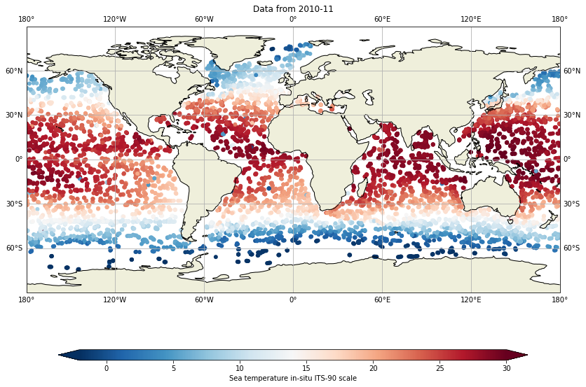
and it is possible to get the WMO of all the platforms measured during this month, together with its data acquisition center. Hence, we can download the netCDF files for each cycle if necessary :
WMOs=np.array([])
DACs=np.array([])
#read all the basins
for basin in ['atlantic_ocean','pacific_ocean','indian_ocean']:
    for iday in range(1,31):
        filein=f"../../Data/{basin}/2020/11/202011{iday:02d}_prof.nc"
        DS=xr.open_dataset(filein)
        #look for the WMO and DAC for each float
        DACs=np.append(DACs,DS.DATA_CENTRE.astype(str).values)
        WMOs=np.append(WMOs,DS.PLATFORM_NUMBER.astype(int).values)

#Keep just the unique set of WMOs
WMOs, indices = np.unique(WMOs, return_index=True)
DACs=DACs[indices]
print(f"During november 2020 {WMOs.shape[0]} Argo floats where active:")
for ip in range(0,WMOs.shape[0],500):
    print(f"{ip} WMO {WMOs[ip]} DAC {DACs[ip]}")
During november 2020 3903 Argo floats where active:
0 WMO 1901302.0 DAC BO
500 WMO 2902785.0 DAC HZ
1000 WMO 3901867.0 DAC IF
1500 WMO 4902549.0 DAC ME
2000 WMO 5904196.0 DAC AO
2500 WMO 5905188.0 DAC CS
3000 WMO 5906066.0 DAC AO
3500 WMO 6902874.0 DAC IF
WMOs=np.array([])
DACs=np.array([])
#read all the basins
for basin in ['atlantic_ocean','pacific_ocean','indian_ocean']:
    for iday in range(1,31):
        filein=f"../../Data/{basin}/2020/11/202011{iday:02d}_prof.nc"
        DS=xr.open_dataset(filein)
        #look for the WMO and DAC for each float
        DACs=np.append(DACs,DS.DATA_CENTRE.astype(str).values)
        WMOs=np.append(WMOs,DS.PLATFORM_NUMBER.astype(int).values)

#Keep just the unique set of WMOs
WMOs, indices = np.unique(WMOs, return_index=True)
DACs=DACs[indices]
fig,ax = plt.subplots(figsize=(15,10))
ax.plot(dayADS.PSAL.transpose(),dayADS.PRES.transpose(),'o-')
ax.set_ylim(0,2000)
ax.invert_yaxis()
ax.set_xlabel(f"{dayADS.PSAL.long_name}")
ax.set_ylabel(f"{dayADS.PRES.long_name}");
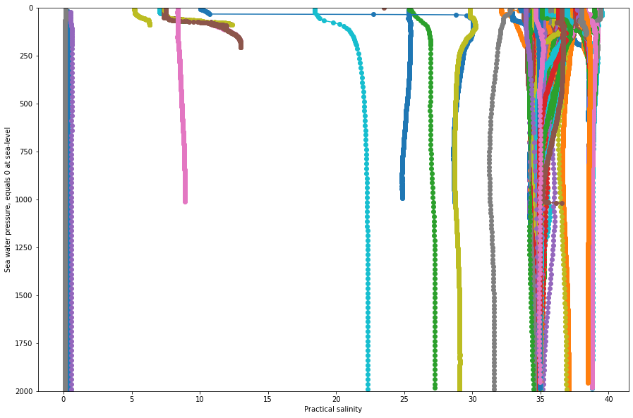
There is some incorrect, or at least suspicious data. In the data variables of the netCDF file, we realise that there are a lot of the _QC variables. In the case of PSAL_QC, it changes for some profiles
fig, ax = plt.subplots(figsize=(20,10))
sc = ax.scatter(dayADS.PSAL, dayADS.PRES, c=dayADS.PSAL_QC, vmin=0, vmax=9, cmap=qcmap)
colorbar_qc(qcmap, ax=ax)
ax.grid()
ax.set_ylim(0,2000)
ax.invert_yaxis()
ax.set_xlabel(f"{dayADS.PSAL.long_name}")
ax.set_ylabel('Pressure')
ax.set_title(f"PSAL {dayADS.PSAL_QC.long_name}");
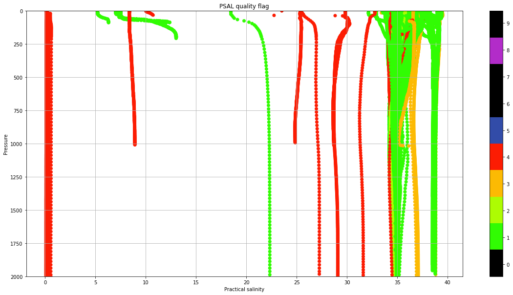
In sections Real Time quality control data and Delayed mode data you may learn everything about the use of this quality control flags, so you can choose the best data available!